?> Options Trading Archives - Page 7 of 17 - projectfinance

Short Iron Condor Explained – The Ultimate Guide

Iron Condor Options Strategy

The short iron condor options strategy is a limited risk strategy consisting of simultaneously selling an out-of-the-money call spread and out-of-the-money put spread in the same expiration date cycle.

Since the sale of a call spread is a bearish strategy and selling a put spread is a bullish strategy, combining the two into a short iron condor results in a directionally neutral position. However, if the stock price moves significantly in either direction, the trade will lose money and also become directional.

The iron condor strategy is very similar to the strangle, except an iron condor has less risk due to using spreads as opposed to naked short options. When selling iron condors, profits come from the passage of time or decreases in implied volatility, as long as the stock price remains between the two breakeven prices of the position.

Care to watch the video instead? Check it out below!

TAKEAWAYS


  • An iron condor consists of selling a put spread (long put/short put) and a call spread (long call/short call) at the same time.


  • Both of these spreads must be of the same width and expiration.


  • Iron condor’s profit when the options sold fall in value.


  • Short iron condors are best suited for market-neutral traders.

  • Maximum loss is greater than maximum profit for most iron condors.


  • High volatility allows traders to collect greater premium from iron condors sold.

Iron Condor Advantages

Iron Condor Advantages

Short Iron Condor Strategy Characteristics

➥ Max Profit Potential: Net Credit Received x 100

➥ Max Loss Potential: (Strike Width of Widest Spread – Net Credit Received) x 100

➥ Expiration Breakevens:

     1. Upper Breakeven = Short Call Strike Price + Net Credit Received

     2. Lower Breakeven = Short Put Strike Price – Net Credit Received

Estimated Probability of Profit: 

Between 50-99% depending on the strikes chosen. The further the short strikes are from the stock price, the higher the probability of profit. However, higher probability of profit comes at the cost of less potential reward.

To demonstrate these characteristics in action, let’s take a look at a hypothetical example to visualize the iron condor strategy’s potential profits and losses at expiration.

P/L Potential at Expiration

In the following example, we’ll construct a short iron condor from the following option chain:

In this case, we’ll sell the 450 put and the 550 call, and buy the 400 put and 600 call. Let’s also assume the stock price is trading for $500 when entering the position:

Initial Stock Price: $500

Short Strikes: $450 short put, $550 short call

Long Strikes: $400 long put, $600 long call

Credit Received From Short Options: $6.15 (450 put) + $7.89 (550 call) = $14.04

Debit Paid for Long Options: $0.72 (400 put) + $1.94 (600 call) = $2.66

Total Credit Received: $14.04 Credit Received – $2.66 Debit Paid = $11.38

The following visual describes the potential profits and losses at expiration when selling this particular iron condor:

Iron Condor Chart

Short iron condor

As illustrated above, the short iron condor strategy realizes its maximum profit potential when the stock price is between the short strikes at expiration, and amounts to the total credit received for selling each spread (multiplied by 100). Additionally, you’ll notice that a short iron condor has a similar risk profile to a short strangle, except the risk of a short iron condor is limited beyond the long options that are purchased.

Regarding loss potential, both the short call spread and short put spread are $50 wide. Because of this, the maximum potential loss is: ($50 strike width – $11.38 credit received) x 100 = $3,862. However, if the call spread were $100 wide (e.g. 550 short call and 650 long call), the maximum loss potential of this iron condor would be: ($100 strike width – $11.62 credit received) x 100 = $8,862. Therefore, an iron condor’s loss potential always depends on the width of the wider spread. When each spread has the same width, the risk of loss is equal on both sides.

The last thing we’ll point out about this graph is that the breakeven prices are both above and below the stock price, which means the stock can trade in a wide range and the short iron condor can be profitable. Because of this, the selling iron condors is a high probability strategy. However, this makes sense since the maximum potential loss is greater than the maximum potential reward (in general).

At this point, you know how the outcomes at expiration when selling iron condors, but what about before expiration? Understanding how profits and losses occur when selling iron condors can be explained by the position’s option Greeks.

Short Iron Condor Trade Examples

To visualize the performance of the iron condor strategy relative to the stock price, let’s look at a few examples of some iron condors that actually occurred. Note that we don’t specify the specific underlying because the concepts transfer to other stocks in the market. Additionally, each example demonstrates the performance of a single iron condor position.

When trading more contracts, the profits and losses in each case will be magnified by the number of iron condors traded.

Let’s do it!

Trade Example #1: Partially Profitable Iron Condor

The first example we’ll look at is a scenario where a trader sells an iron condor, but the stock price is between the short call option and long call option at expiration. In this scenario, maximum profit will not be realized, but the strategy can still be profitable if the stock price is below the upper breakeven price.

Here are the trade details:

Initial Price of The Underlying Stock: $202.31

Strikes and Expiration: Long 182 Put and 215 Call; Short 196 Put and 208 Call; All options expiring in 72 days

Net Premium Received for Short Options: $4.18 for the 196 put + $2.82 for the 208 call = $7.00 in premium collected

Net Premium Paid for Long Options: $1.79 for the 182 put + $0.78 for the 215 call = $2.57 in premium paid

Net Credit: $7.00 premium collected – $2.57 premium paid = $4.43 net credit

Breakeven Prices: $191.57 and $212.43 ($196 – $4.43 and $208 + $4.43)

Maximum Profit Potential: $4.43 net credit x 100 = $443

Maximum Loss Potential (Upside): ($7-wide call spread – $4.43 net credit) x 100 = $257

Maximum Loss Potential (Downside): ($14-wide put spread – $4.43 net credit) x 100 = $957

As mentioned earlier, the maximum loss potential of an iron condor depends on the wider spread. In this example, the short call spread is $7 wide and the short put spread is $14 wide. Because of this, the maximum loss potential of this iron condor occurs when the stock price collapses through the short put spread. More specifically, this trade has $257 in loss potential on the upside and $957 in potential losses on the downside. Consequently, this particular short iron condor position has a slightly bullish bias.

Let’s see what happens!

Iron Condor #1 Trade Results

As we can see, this short iron condor position performed well because the stock price remained between the position’s breakeven points over the entire period. 

With the price of the iron condor below the initial sale price nearly the entire period, the trader in this example had many opportunities to close the trade early for profits. To close an iron condor before expiration, a trader can simultaneously buy back the short options and sell the long options at their current prices. 

For example, if the trader in this example closed the iron condor for $3.00, they would have locked in a profit of $143: ($4.43 initial iron condor sale price – $3.00 closing price) x 100 = +$142.

At expiration, the short 208 call was worth $2.50 because the stock price was trading for $210.50. Since all of the other options expired worthless, the final value of the iron condor is $2.50. With an initial sale price of $4.43, the profit at expiration is: ($4.43 – $2.50) x 100 = +$193.

Regarding a share assignment, this particular trader would be assigned -100 shares of stock if they did not close the in-the-money short call before expiration. If the trader did not want a short stock position, the short call would need to be bought back before expiration. However, there’s always a chance that the trader could get assigned early on the short call.

Ok, so you’ve seen a partially profitable iron condor example. Next, we’ll take a look at a scenario where a short iron condor realizes the maximum potential loss.

Trade Example #2: Maximum Loss Iron Condor

In the following example, we’ll investigate a situation where the stock price rises continuosly and is above the short call spread at expiration.

Here are the details:

Initial Stock Price: $121.45

Strikes and Expiration: Long 115 Put and 128 Call; Short 119 Put and 124 Call; All options expiring in 46 days

Premium Collected for Short Options: $1.25 for the 119 put + $1.05 for the 124 call = $2.30 in premium collected

Premium Paid for Long Options: $0.39 for the 115 put + $0.38 for the 128 call = $0.77 in premium paid

Net Credit: $2.30 premium collected – $0.77 premium paid = $1.53 net credit

Breakeven Prices: $117.47 and $125.53 ($119 – $1.53 and $124 + $1.53)

Maximum Profit Potential: $1.53 net credit x 100 = $153

Maximum Risk: ($4-wide spreads – $1.53 net credit) x 100 = $247

In this example, both the short call spread and short put spread are $4 wide, so the risk is equal on both sides of the trade.

Let’s take a look at the trade’s performance:

iron condor trade example

Iron Condor #2 Trade Results

As we can see in this example, the stock price rallied from $121 to over $130 during the duration of this trade. Since the stock price increased steadily after entering the trade, the position suffered losses and was never profitable.

At expiration, the stock price was above $128, which means the short 124/128 call spread was entirely in-the-money (ITM) and was therefore worth $4, which is the width of the spread.

On the other hand, the short 119/115 put spread expired worthless because both put options were out-of-the-money (OTM). 

With the iron condor being worth $4 at expiration, the trader’s loss in this example is $247 per iron condor, as the position was sold for $1.53 but ended at $4.00.

Trade Example #3: Max Profit Iron Condor

In the final example, we’ll look at a scenario where a short iron condor trader only makes full profit at expiration. The maximum profit of an iron condor occurs when the stock price is between the short strikes at expiration.

Here are the trade details:

Initial Stock Price: $574.81

Strikes and Expiration: Long 505 Put and 645 Call; Short 535 Put and 615 Call; All options expiring in 46 days

Premium Collected for Short Options: $11.75 for the 535 put + $10.40 for the 615 call = $22.15 in premium collected

Premium Paid for Long Options: $6.03 for the 505 put + $4.47 for the 645 call = $10.50 in premium paid

Net Credit: $22.15 premium collected – $10.50 premium paid = $11.65 net credit

Breakeven Prices: $523.35 and $626.65 ($535 – $11.65 and $615 + $11.65)

Maximum Profit Potential: $11.65 net credit x 100 = $1,165

Maximum Loss Potential: ($30-wide spreads – $11.65 net credit) x 100 = $1,835

Let’s see this historical trade’s performance!

iron condor options

Iron Condor #3 Trade Results

In this case, the stock price collapsed immediately after the iron condor was sold. As a result, the iron condor price jumped from $11.65 to over $20.00, which translated to a loss of over $850 for the iron condor seller. Fortunately, the stock price rallied back between the position’s short strikes and the position decayed as expiration approached.

Finally, at expiration, all of the options expired worthless since the stock price was between the short strikes of each spread. With an initial sale price of $11.65, the profit on this trade is $1,165: ($11.65 sale price – $0 expiration price) x 100 = +$1,165.

Curious about the “Iron Butterfly” strategy? Learn it here!

Final Word

Let’s review what we have learned:

  • An iron condor consists of selling both a put spread (long put/short put) and a call spread (long call/short call) simultaneously
  • Both of these spreads must be of the same width and expiration
  • Iron condor’s profit when the options sold decrease in value
  • Short iron condors are best suited for market-neutral traders
  • Most iron condors have a greater than 50% chance of success
  • Maximum loss is greater than maximum profit for most iron condors
  • A high volatility environment allows traders to collect more premium from iron condors sold
  • Iron condors with 30-60 days to expiration are ideal as this time frame allows traders to profit from time decay, or the Greek “theta

Options trading involves risks. To learn more about these risks, please read the risks of standardized options from The OCC.

Short Iron Condor FAQs

The long iron condor is the exact opposite trade of the short iron condor. Long iron condors are purchased for a debit while short iron condors are sold for a net credit. 

When you buy an iron condor, you believe the underlying stock will make a large directional move either up or down. Short iron condors profit in a neutral market. 

Short iron condors can go into expiration as long as both the short call option and short put option are safely out-of-the-money. If either of these legs is close to being in-the-money as expiration nears, it is best practice to trade out of these options. 

Chris Butler portrait

Short Straddle Explained – The Ultimate Guide

Short Straddle Chart

The short straddle is an options strategy that consists of selling call and put option on a stock with the same strike price and expiration date.

Most of the time, a short straddle trader will sell the at-the-money options. Since the sale of an at-the-money call is a bearish strategy, and selling a put is a bullish strategy, combining the two into a short straddle results in a directionally neutral position. However, as the stock price changes, the trade will become directional and can suffer significant losses.

When selling straddles, profits come from the passage of time or decreases in implied volatility, as long as the stock price remains within the breakeven points of the position. Selling straddles is very similar to selling strangles, with the only difference being that the short call and put share the same strike price.

TAKEAWAYS

  • The short straddle is best suited for neutral, or “sideways” market direction.

  • One short call and one short put comprise this strategy.

  • The loss on this strategy is infinite  because of the short call sold.

  • Total profit is limited to the credit received.

Short Straddle Strategy Characteristics

Max Profit Potential: Total Credit Received x 100

Max Loss Potential: Unlimited

Expiration Breakevens:

➥Upper Breakeven = Strike Price + Total Credit Received

➥Lower Breakeven = Strike Price – Total Credit Received

Estimated Probability of Profit: Generally between 50-60%.

To demonstrate these characteristics in action, let’s take a look at a basic example and visualize the position’s potential profits and losses at expiration.

Short Straddle Profit/Loss Potential at Expiration

In the following example, we’ll construct a short straddle from the following option chain:

In this case, we’ll sell the 250 call and 250 put. Let’s also assume the stock price is $250 when entering the trade.

Initial Stock Price: $250

Short Strikes Used: 250 put, 250 call

250 Put Sale Price: $15.10

250 Call Sale Price: $15.20

Total Credit Received: $15.10 + $15.20 = $30.30

The following visual describes the potential profits and losses at expiration when selling this particular straddle:

Short Straddle Chart

Short Straddle

As illustrated here, a short straddle realizes maximum profit when the stock price is trading exactly at the short strike at expiration. Because of this, achieving maximum profit on a short straddle is very unlikely

However, since a short straddle collects the most extrinsic value compared to any other option selling strategy, taking partial profits on a short straddle can lead to more profits than making maximum profit on other less aggressive strategies.

The sections below explain the why behind the profit/loss levels at various stock prices at the time of expiration:

Stock Price Below the Lower Breakeven Price ($219.70):

The 250 call expires worthless but the short 250 put has more intrinsic value than the entire straddle was sold for ($30.30), and therefore the straddle seller realizes a loss.

Stock Price Between the Lower Breakeven and the Short 250 Put ($219.70 to $250):

The 250 put has intrinsic value, but not more than the premium the trader collected when selling the straddle. The 250 call expires worthless. Consequently, the short straddle position is profitable.

Stock Price Between the Short Call Strike and the Upper Breakeven ($250 to $280.30):

The 250 call has intrinsic value, but not more than the premium the trader collected when selling the straddle. The 250 put expires worthless. Consequently, the short straddle position is profitable.

Stock Price Above the Upper Breakeven ($280):

The 250 put expires worthless but the 250 call has more intrinsic value than the straddle was sold for, and therefore the short straddle position is not profitable. Since the stock price can rise indefinitely, the short call (and consequently the entire short straddle) has unlimited loss potential.

Great job! You’ve learned the general characteristics of the short straddle strategy. Now, let’s go through some visual trade examples to show you how selling straddles really works.

Short Straddle Trade Examples

To visualize the performance of straddles relative to the stock price, let’s look at a few examples of real straddles that recently traded. Note that we don’t specify the underlying, since the same concepts apply to short straddles on any stock. Additionally, each example demonstrates the performance of a single straddle positionWhen trading more contracts, the profits and losses in each case will be magnified by the number of straddles traded.

Let’s do it!

Trade Example #1: Highly Profitable Short Straddle Trade

The first example we’ll look at is a situation where the stock price trades in a tight range after an at-the-money straddle is sold, resulting in plenty of profits.

Here are the trade entry details:

Initial Stock Price: $210.72

Initial Implied Volatility: 15%

Strikes and Expiration: 211 put and 211 call expiring in 77 days

Straddle Sale Price: $5.46 for the put and $4.32 for the call = $9.78 total credit

Breakeven Prices: $201.22 and $220.78 ($211 – $9.78 and $211 + $9.78)

Maximum Profit Potential: $9.78 net credit x 100 = $978

Maximum Loss Potential: Unlimited

Let’s visualize what happens that allows this trade to profit!

Selling a straddle

Short Straddle #1 Trade Results

As you can see, selling straddles can be highly profitable when the stock price doesn’t rise or fall quickly with magnitude. In this case, the stock price traded near the short strike the entire time, leading to profits from time decay. Implied volatility remained near 15% the entire period, so a change in implied volatility really wasn’t a factor here.

In this example, the straddle price continously fell, presenting many opportunities for the short straddle trader to close the position early for profits. To lock in the profits or losses on a short straddle position, the short options can be simultaneously bought back at their current prices. For example, if the trader in this position bought back the straddle for $5.00, they would have locked in $478 in profits: ($9.78 initial sale price – $5.00 closing price) x 100 = +$478.

At expiration, the stock price was above $211, which means the short call was in-the-money and the short put was out-of-the-money. However, the short 211 call only had $1.50 of intrinsic value at expiration, which results in a $828 profit for the straddle seller: ($9.78 sale price – $1.50 expiration value) x 100 = +$828.

Trade Example #2: Large Loss

In the next example, we’ll look at how a short straddle performs when the stock price falls significantly. In particular, we’ll examine a short straddle on a stock in late 2008.

Here are the trade details:

Initial Stock Price: $126.20

Initial Implied Volatility: 23%

Strikes and Expiration: 126 put and 126 call expiring in 78 days

Straddle Sale Price: $5.18 for the put and $5.07 for the call = $10.25 total credit

Breakeven Prices: $115.75 and $136.25 ($126 – $10.25 and $126 + $10.25)

Maximum Profit Potential: $10.25 net credit x 100 = $1,025

Maximum Loss Potential: Unlimited

Let’s visualize what goes wrong, causing the trade to lose money:

short straddle options

Short Straddle #2 Trade Results

As you can see here, the short straddle position did ok in the first 40 days of the period. However, the stock price suddenly collapsed from $125 to $95. At the same time, implied volatility in the expiration cycle of the short straddle spiked to over 75%. Consequently, the price of the 126 straddle surged in price to $35. With an initial sale price near $10, the loss is $2,500 per short straddle when the straddle is worth $35. 

If the trader wanted to take losses before expiration, the straddle can be bought back at its current price. For example, if the straddle was bought back for $25, the trader would have locked in $1,475 in losses: ($10.25 initial sale price – $25 closing price) x 100 = -$1,475.

At expiration, the stock price was $31 below the straddle’s strike price of $126, which translates to $31 of intrinsic value for the 126 put and $0 of intrinsic value for the 126 call. Because of this, the expiration loss for the straddle seller is $2,075: ($10.25 initial sale price – $31 final straddle value) x 100 = -$2,075.

Changes in a Short Straddle's Delta/Directional Exposure

In addition to demonstrating the potential losses from selling straddles, this example serves as an excellent demonstration of how a straddle’s position delta can change rather quickly.

As mentioned earlier, a short straddle position has negative gamma, which means that as the stock price trends in one direction, the delta (directional risk) of the position will grow in the opposite direction. 

For example, if the stock price increases, the delta of a short straddle position will become more negative, resulting in a bearish position. Conversely, when the stock price decreases, the delta of a short straddle position will grow more positive, resulting in a bullish position.

Let’s visualize the concept of negative gamma using the same example as above:

Straddle vs Delta

straddle vs delta

As visualized here, the position delta of the short straddle moves inversely with the stock price. When the stock price increases, the position delta becomes more negative, which means the position is more bearish. When the stock price decreases, the position delta becomes more positive, which means the position is more bullish. Intuitively, this should make sense because the maximum profit potential of a short straddle occurs when the stock price is right at the strike price.

Therefore:

When the stock price falls below the strike price, the position becomes bullish because the ideal scenario is for the stock price to rise back up to the strike price.

When the stock price rises above the strike price, the position becomes bearish because the best case scenario is for the stock price to fall back down to the strike price.

Trade Example #3: Breakeven Short Straddle

In the final example, we’ll look at a scenario where a short straddle trader doesn’t make or lose much money, which occurs when the stock price is near one of the straddle’s breakeven prices at expiration.

Here are the trade details:

Initial Stock Price: $210.56

Strikes and Expiration: 211 put and 211 call expiring in 60 days

Straddle Sale Price: $4.83 for the put and $3.51 for the call = $8.34 total credit

Breakeven Prices: $202.66 and $219.34 ($211 – $8.34 and $211 + $8.34)

Maximum Profit Potential: $8.34 net credit x 100 = $834

Maximum Loss Potential: Unlimited

Let’s see what happens that causes the trade to break even:

selling straddle options

Short Straddle #3 Trade Results

As we can see here, the stock price fell significantly after the short straddle was entered. As a result, the position had losses over the entire period. At the worst point, the loss on the short straddle was nearly $1,700.

Fortunately, the stock price rallied back to the short straddle’s lower breakeven price. At expiration, the 211 put had slightly less than $8.34 of intrinsic value, which means the position squeaked out a tiny profit because the initial straddle sale price was $8.34.  

Regarding a share assignment, the short 211 put is in-the-money at expiration, which means the trader would be assigned +100 shares of stock if the put was held through expiration (if not already assigned shares early).

Final Word

Let’s briefly review a few of the key concepts we have learned:

  • When the stock prices breaks one of the strike prices sold, the straddle can experience significant losses. 
  • In the straddle, the most you can ever make is the credit received. 
  • Short straddles have a negative gamma, which has an inverse relationship with delta.

Curious how the strangle compares to the straddle? Check out our article here, Straddles vs Strangles.

Chris Butler portrait

Short Strangle Explained – The Ultimate Visual Guide

Short strangle chart

The short strangle is an options strategy that consists of selling an out-of-the-money call option and an out-of-the-money put option in the same expiration cycle.

Since selling a call is a bearish strategy and selling a put is a bullish strategy, combining the two into a short strangle results in a directionally neutral position.

However, if the stock price moves towards one of the short strikes, the trade becomes directional and can suffer significant losses. When selling strangles, profits come from the passage of time or decreases in implied volatility, as long as large stock price movements in one direction do not occur.

TAKEAWAYS

  • The short strangle is best suited for neutral, or “sideways” market direction.

  • One short call and one short put comprise this strategy.

  • The loss on this strategy is infinite  because of the short call sold.

  • Total profit is limited to the credit received.

Short Strangle Strategy Characteristics

Before getting into examples, let’s look at the short strangle’s general characteristics:

➥Max Profit Potential: Total Credit Received x 100

➥Max Loss Potential: Unlimited

➥Expiration Breakevens:

Upper Breakeven = Call Strike Price + Total Credit Received

Lower Breakeven = Put Strike Price – Total Credit Received

➥Estimated Probability of Profit: Between 50-99% depending on the options sold. However, the higher the probability of profit, the lower the potential reward.

To demonstrate these characteristics in action, let’s take a look at a basic example and visualize the position’s potential profits and losses at expiration.

Expiration Profit/Loss Potential

In the following example, we’ll construct a short strangle position using the following option chain:

In this case, we’ll sell the 190 put and the 210 call. Let’s also assume the stock price is trading for $200 when the strangle is sold.

Initial Stock Price: $200

Short Strikes Used: 190 put, 210 call

190 Put Sale Price: $3.78

210 Call Sale Price: $4.31

Total Credit Received: $3.78 + $4.31 = $8.09

The following visual describes the potential profits and losses at expiration when selling this particular strangle:

Short Strangle Chart

short strangle chart

As illustrated here, a short strangle realizes the maximum profit potential when the stock price is between the short strikes at expiration because each option expires worthless. Additionally, the collection of premium extends the breakeven prices beyond the short strikes of the trade, which means the stock price can trade beyond one of the short strikes and the position can still be profitable.

More specifically, the strangle will be profitable at expiration as long as one of the options isn’t in-the-money by more than the total credit received from selling the strangle.

Short Strangle Trade Examples

To visualize the performance of strangles relative to the stock price, let’s look at a few examples of real strangles that recently traded. Note that we don’t specify the underlying, since the same concepts apply to short strangles on any stock. Additionally, each example demonstrates the performance of a single strangle position. 

When trading more contracts, the profits and losses in each case will be magnified by the number of strangles traded.

Trade Example #1: Maximum Profit Strangle

The first example we’ll look at is a situation where a hypothetical trader sells a strangle with a call and put that have deltas near ±0.20.

With a delta near ±0.20, the call and put both have an estimated 20% probability of expiring in-the-money, respectively. Because of this, the strangle as a whole has an approximate 40% probability of expiring in-the-money, which translates to a 60% probability of expiring out-of-the-money.

Here are the trade details:

Initial Stock Price: $212.44

Initial Implied Volatility: 14%

Strikes and Expiration: 201 put and 219 call expiring in 63 days

Strangle Sale Price: $1.75 for the put and $0.83 for the call = $2.58 total credit

Breakeven Prices: $198.42 and $221.58 ($201 – $2.58 and $219 + $2.58)

Maximum Profit Potential: $2.58 net credit x 100 = $258

Maximum Loss Potential: Unlimited

Let’s examine this historical trade’s performance:

short strangle trade

Strangle #1 Trade Results

As you can see, selling strangles is profitable as long as the stock price doesn’t rise or fall significantly. In this case, the stock price was between the short strikes the entire time, leading to profits from time decay. The options decrease in price as time passes because there is a diminishing probability that each option will expire in-the-money.

In other words, when the stock price remains between the short strikes, the probability that the call or put expire in-the-money decreases as time passes, which explains the strangles decaying price.

At around 18 days to expiration, you’ll notice that the strangle’s price rises from $0.50 to $2.00. The strangle’s price increase can be explained by the sharp stock price decrease and the subsequent increase in implied volatility to 21% (not visualized in the chart). However, the short strangle position was still profitable because the profits from time decay at that point were greater than the losses from the movements in the stock price and implied volatility.

In this example, the strangle price was below the initial sale price the entire period. As a result, the trader had ample opportunity to close the position before expiration to lock in profits. To close a short strangle, the short options need to be bought back at their current prices. For example, if the strangle trader bought back the strangle for a $1.00 debit, they would have locked in profits of $158: ($2.58 initial sale price – $1.00 closing price) x 100 = +$158.

With the stock price between the short strikes at expiration, the 201 put and 219 call expired worthless, resulting in the maximum profit potential of $258 for the strangle seller.

The example above demonstrates what can go right when selling strangles. In the next demonstration, we’ll look at a scenario where a short strangle position turns into a big loser.

Trade Example #2: Significant Loss

In the last example, you saw how a sharp decrease in the stock price towards the short put strike could lead to an increase in the price of the strangle. In this example, we’ll examine what happens to the price of a strangle when the stock price collapses through the short put strike. Additionally, we’ll investigate how the position’s directional exposure (delta) changes.

Here are the trade details:

Initial Stock Price: $524

Initial Implied Volatility: 26%

Strikes and Expiration: 495 put and 555 call expiring in 39 days

Strangle Sale Price: $6.35 for the put and $6.20 for the call = $12.55 total credit

Breakeven Prices: $482.45 and $567.55 ($495 – $12.55 and $555 + $12.55)

Maximum Profit Potential: $12.55 net credit x 100 = $1,255

Maximum Loss Potential: Unlimited

Strangle #2 Trade Results

As you can see here, the short strangle position did not experience continuous profits like the previous example. Between 32 and 24 days to expiration, the stock price collapsed from nearly $540 to $460, which is $35 below the short put’s strike price of $495. At the same time, implied volatility increased from 26% to 54%. As a result of the directional move and shift in implied volatility, the price of the put surged to $42 while the call price fell to $2. Because of this, with 25 days to expiration, the short strangle trader has the following profits and losses on each option:

➜ Short Call Profit: ($6.20 sale price – $2.00 current price) x 100 = $420

➜ Short Put Loss: ($6.35 sale price – $42.00 current price) x 100 = -$3,565

​Net Loss: $420 profit – $3,465 loss = -$3,145

When the stock price collapses through the short put strike before expiration, the loss on the short put will likely be greater than the profit on the short call, resulting in a net loss for a strangle seller. 

On the other hand, when the stock price increases through the short call strike before expiration, the loss on the short call will likely be greater than the profit on the short put, which also results in a net loss for the short strangle trader.

Fortunately, in this example, the stock price regained its losses and was between the short strikes at expiration, leading to the maximum profit of $1,255 for the strangle seller.

As mentioned previously, the strangle trader in this example could have closed the position early to lock in losses. For example, if the trader wanted to cut the losses when the strangle traded up to $30, they could have bought back the strangle for $30 and locked in losses of $1,745: ($12.55 initial sale price – $30 closing price) x 100 = -$1,745.

Negative Gamma Demonstration

In addition to demonstrating the potential losses from selling strangles, the example below serves as a great demonstration of how a strangle’s directional risk can change rather quickly. A short strangle position has negative gamma, which means that as the stock price trends in one direction, the position delta (directional exposure) of the position will grow in the opposite direction.

For example, if the stock price increases, the delta of a short strangle position will become more negative, resulting in a bearish position. Conversely, when the stock price decreases, the delta of a short strangle position will grow more positive, resulting in a bullish position.

Let’s visualize the concept of negative gamma using the same example as above:

Short Strangle and Delta

strangle greeks

As visualized here, the position delta of the short strangle moves inversely with the stock price. When the stock price increases, the position delta becomes more negative. When the stock price decreases, the position delta becomes more positive. Therefore, when trading neutral trading strategies, understand that the positions can become very directional in a short period of time.

In this example, the position delta started near zero because a +0.20 delta call and -0.20 delta put were sold (respective position deltas of -20 and +20). However, when the stock price collapsed, the put delta approached -1 while the call delta approached zero. As a result, the position delta grew positively because being short a negative delta option (a put) results in a positive position delta. 

In the case of this 495/555 strangle, the position delta increased from -20 to +70 when the stock price fell from $540 to $460. With a position delta of -20, the short strangle has the directional exposure of being short 20 shares of stock. On the other hand, with a position delta of +70, the short strangle has the directional exposure of being long 70 shares of stock.

The moral of the story is that a short strangle is not likely to remain directionally neutral when the stock price changes. Because of this, the delta of a short strangle should be monitored closely, especially near expiration.

Trade Example #3: Partially Profitable Short Strangle

In the final example, we’ll look at a scenario where a short strangle trader only makes a partial profit at expiration. Partial profits occur when the stock price is between one of the short strikes and the breakeven price on that side. Here’s the setup:

Initial Stock Price: $108.29

Strikes and Expiration: 103 put and 111 call expiring in 44 days

Strangle Sale Price: $1.40 for the put and $1.82 for the call = $3.22 total credit

Breakeven Prices: $99.78 and $114.22 ($103 – $3.22 and $111 + $3.22)

Maximum Profit Potential: $3.22 net credit x 100 = $322

Maximum Loss Potential: Unlimited

Let’s see what happens!

Strangle #3 Trade Results

As we can see here, the stock price fell below the short put strike shortly after the trade was entered, and remained below the put for most of the period. Consequently, this short strangle did not do particularly well, and was worth almost twice the entry credit at one point. However, the position was partially profitable at expiration because the stock price was above the lower breakeven price.

With the stock price at $101.50 at expiration, the 103 put expired worth $1.50, resulting in a profit of $172: ($3.22 initial sale price – $1.50 strangle price at expiration) x 100 = +$172.

Regarding a share assignment, the 103 short put would expire to +100 shares of stock if held through expiration. To avoid a share assignment, the put would need to be bought back before expiration. However, it’s always possible that the trader is assigned early on the in-the-money short put before expiration.

Final Word

Let’s briefly review a few of the key concepts we have learned:

  • When the stock prices breaks one of the strike prices sold, the strangle can experience significant losses. 
  • In the strangle, the most you can ever make is the credit received. 
  • Short strangles have a negative gamma, which has an inverse relationship with delta.
Chris Butler portrait

Synthetic Long Stock & Synthetic Short Stock W/ Visuals

▼ The synthetic short stock options strategy consists of simultaneously selling a call option and buying the same number of put options at the same strike price.

Both options must be in the same expiration cycle. As the strategy’s name suggests, a synthetic short stock position replicates shorting 100 shares of stock. 

▲ The synthetic long stock position consists of simultaneously buying a call option and selling the same number of put options at the same strike price. Both options must be in the same expiration cycle. As the strategy’s name suggests, a synthetic long stock position replicates buying and holding 100 shares of stock. 

By owning a call option and selling a put option at the same strike price, the synthetic long position’s delta exposure will be +100. Compared to buying shares of stock, a trader may be able to enter a synthetic long stock position with a lower margin requirement than buying shares.

        TAKEAWAYS


  • The profit/loss profile of a “synthetic short” mirrors that of short stock and is thus bearish.

  • The strategy consists of 1.) short call and 2.) long put.

  • Because of the short call, risk on this strategy is unlimited.

  • Max profit occurs on the long put side, and happens if the stock goes to zero.

  • Because of options leverage, the synthetic short options strategy can be a cheaper alternative than shorting stock.

  • The synthetic long stock trade is an advanced options trading strategy.

  • The position is created from buying a call option and selling a put option of the same strike.

  • The position is suited for very bullish investors who don’t want to pay for the stock.

  • Due to the short putmax loss in this strategy is great.

Synthetic Short Stock Strategy Characteristics

Let’s go over the synthetic short stock strategy general characteristics:

Max Profit Potential

If the synthetic is entered for a debit: (Strike Price – Debit) x 100

If the synthetic is entered for a credit: (Strike Price + Credit) x 100

Max Loss Potential: Unlimited

Expiration Breakeven

If the synthetic is entered for a debit: Strike Price – Debit Paid

If the synthetic is entered for a credit: Strike Price + Credit Received

To demonstrate these characteristics in action, let’s take a look at a basic example.

Profit/Loss Potential at Expiration

In the following example, we’ll replicate a short share position from the following call and put options:

In this example, we’ll simultaneously sell the 100 call and buy the 100 put. When trading synthetic stock positions, you can use any strike price, as long as you purchase the put and sell the call at that strike (in the same expiration cycle).

We choose to use the at-the-money options because they are the most actively traded options, which benefits traders in terms of liquidity.

Lastly, let’s assume the stock price is trading for $100 when entering the position:

Initial Stock Price: $100

Synthetic Short Stock Setup: Short 100 call for $3.53; Long 100 put for $3.44

Credit Received for Synthetic: $3.53 received – $3.44 paid = $0.09

Breakeven Price: $100 strike price + $0.09 credit received = $100.09

As you can see, the position’s breakeven is only $0.09 above the current stock price. The difference is explained by carrying costs that are priced into the options. In this example, the carrying costs stem from the risk-free interest rate, as the stock in this example does not pay any dividends.

The following visual describes the position’s potential profits and losses at expiration:

Synthetic Short Chart

synthetic short chart

As we can see here, the risk profile of a synthetic short stock position is identical to an actual short stock position. The only difference is the breakeven price, which is miniscule. To be profitable when trading synthetic short stock positions, the stock price must decrease from the point of entry.

Great job! You’ve learned the general characteristics of the synthetic short stock position. Now, let’s go through a real trade example and visualize the performance of the position through time.

Synthetic Short Stock Trade Example

To bring the previous section to life, we’re going to look at a real synthetic short stock example and visualize the position’s performance over time.

Here are the trade details:

Initial Stock Price: $109.82

Strikes and Expiration: Short 110 call for $4.13; Long 110 put for $4.28; Both options expiring in 45 days

Net Debit: $4.28 in premium paid – $4.13 in premium collected = $0.15 net debit

Breakeven Price: $110 strike price – $0.15 net debit = $109.85

Maximum Profit Potential: $109.85 x 100 = $10,985 (stock price at $0)

Maximum Loss Potential: Unlimited

Let’s see what happens!

synthetic short stock

Synthetic Short Trade Results

As you can see, the performance of a short stock position and synthetic short stock position are identical. When the stock price increases from the point of entry, both positions have losses. Conversely, when the stock price falls below the entry price, both positions are profitable.

Now that we’ve learned the synthetic short strategy, let’s move on to the synthetic long options strategy!

Synthetic Long Stock - Strategy Characteristics

Let’s go over the synthetic long stock strategy’s general characteristics:

➦ Max Profit Potential: Unlimited

➦ Max Loss Potential: 

  If the synthetic is entered for a debit: (Strike Price + Debit) x 100

  If the synthetic is entered for a credit: (Strike Price – Credit) x 100

➦ Expiration Breakeven:

 If the synthetic is entered for a debit: Strike Price + Debit Paid

 If the synthetic is entered for a credit: Strike Price – Credit Received

➦ Estimated Probability of Profit: Approximately 50% because a synthetic long stock replicates owning shares of stock.

To demonstrate these characteristics in action, let’s take a look at a basic example.

Profit/Loss Potential at Expiration

In the following example, we’ll replicate a long share position from the following option chain:

In this example, we’ll simultaneously buy the 100 call and sell the 100 put. When trading synthetic stock positions, you can use any strike price because the breakeven of each position will be the same. We choose to use the at-the-money options because they are the most actively traded options, which benefits traders in terms of liquidity. Lastly, let’s assume the stock price is trading for $100 when entering the position:

Initial Stock Price: $100

Synthetic Long Stock Setup: Long 100 call for $3.53; Short 100 put for $3.44

Debit Paid for Synthetic: $3.53 paid – $3.44 collected = $0.09

Breakeven Price$100 strike price + $0.09 debit paid = $100.09

As you can see, the position’s breakeven is only $0.09 above the current stock price. The difference is explained by carrying costs that are priced into the options. In this example, the carrying costs stem from the risk-free interest rate, as the stock in this example does not pay any dividends.

The following visual describes the position’s potential profits and losses at expiration: 

synthetic long stock options

As we can see here, the risk profile of a synthetic long stock position is identical to an actual long stock position. The only difference is the breakeven price, which is miniscule. To be profitable when trading synthetic long stock positions, the stock price must increase from the point of entry.

Nice job! You’ve learned the general characteristics of the synthetic long stock position. Now, let’s go through a real trade example and visualize the performance of the position through time.

Synthetic Long Stock Trade Example

To bring the previous section to life, we’re going to look at a real synthetic long stock example and visualize the position’s performance over time. Here’s the trade setup:

Initial Stock Price: $109.82

Strikes and Expiration: Long 110 call for $4.13; Short 110 put for $4.28; Both options expiring in 45 days

Net Credit: $4.28 in premium collected – $4.13 in premium paid = $0.15 net credit

Breakeven Price: $110 strike price – $0.15 net credit = $109.85

Maximum Profit Potential: Unlimited

Maximum Loss Potential: $109.85 x 100 = $10,985

Let’s see what happens!

synthetic long stock example

As you can see, the performance of a long stock position and synthetic long stock position are identical. When the stock price increases from the point of entry, both positions are profitable. Conversely, when the stock price falls below the entry price, both positions have losses.

Final Word

Hopefully, this short guide has helped you better understand synthetic options strategies! Let’s review what we have learned:

  • The synthetic short stock strategy can be a cheaper alternative to selling a stock.
  • Because of the short call, the synthetic short position has infinite risk. 
  • Be sure to choose liquid options when determining your strike price!

  • The synthetic long stock strategy is referred to as “synthetic” because it mirrors a stock position of 100 shares.
  • For small accounts wanting upside exposure, synthetic longs are a great alternative to buying more expensive stock.
  • Because of the short, unhedged put, max loss is great for synthetic long positions.
Chris Butler portrait

Bear Call Spread Option Strategy (Guide w/ Visuals)

Bear Call Spread Graph

The bear call spread (selling a call spread – also known as a “short” call spread) is a bearish options strategy that consists of simultaneously selling a call and buying a call at a higher strike price (same expiration cycle). 

The strategy builds on a naked short call by purchasing a call at a higher strike to reduce the risk of the position.

TAKEAWAYS

  • The short call spread is a great strategy for risk-conscious traders who are either bearish or neutral on the market (and sometimes mildly bullish).

  • The long call portion of this strategy caps losses.

  • On a short call spread, the max loss is the difference between the strike prices minus the net credit received.

  • The short call strategy profits from time decay on the short strike price.

Bear Call Spread Strategy Characteristics

Let’s quickly go over the strategy’s general characteristics:

➟Maximum Profit Potential: Credit Received x 100

➟Maximum Loss Potential: (Width of Call Strikes – Credit Received) x 100

➟Expiration Breakeven Price: Short Call Strike Price + Credit Received

To better understand each of these characteristics, we’re going to look at a basic short call spread example.

Bear Call Spread Profit/Loss Potential at Expiration

In the following example, we’ll construct a short call spread from the following option chain:

In order to construct a short call spread, we’ll have to sell a call while also purchasing a call at a higher strike price. In this example, we’ll sell the 310 call for $8 and purchase the 320 call for $5. Let’s also say that the stock price is trading for $300 at the time of selling the spread:

Initial Stock Price: $300

Call Spread Setup: Sell 310 call for $8, Buy 320 call for $5

Call Spread Sale Price: $8 Received – $5 Paid = $3 Net Credit

If a trader sells this call spread, their potential profits and losses at expiration are described by the following visual:

Bear Call Spread Chart

The following table describes various scenarios of this bear call spread example at expiration:

Stock Price Below the Short Call Strike Price (Below $310)

Both call options in the spread expire worthless, resulting in an $800 profit on the short 310 call, and a $500 loss on the long 320 call. The net profit for the call spread seller is $300: ($3 initial spread sale price – $0 spread price at expiration) x 100 = +$300.

Stock Price Between the Short Call Strike Price and the Breakeven Price (Between $310 and $313)

The short 310 call expires with intrinsic value, but not more than the $3 credit that was collected from selling the spread. Because of this, the short call spread position is partially profitable. Additionally, the trader will be assigned -100 shares of stock for $310 per share if the short call is held through expiration.

Stock Price Between the Breakeven Price and the Long Call Strike Price (Between $313 and $320)

The short 310 call expires with more intrinsic value than the call spread was initially sold for, and therefore the position realizes losses. Additionally, the trader will be assigned -100 shares of stock for $310 per share if the short call is held through expiration.

Stock Price Above the Long Call Strike Price (Above $320)

The 310/320 call spread is worth its maximum value of $10, and therefore the seller of the call spread realizes the maximum loss potential. Since the spread was initially sold for $3, the loss is $700: ($3 sale price – $10 spread price at expiration) x 100 = -$700.

Great job! You know the potential outcomes for a short call spread at expiration, but what about before expiration?

To demonstrate to you how short call spreads perform over time, let’s look at some historical trade examples so you can see how the strategy performs in different scenarios.

Bear Call Spread Trade Examples

To visualize the performance of various short call spread positions, let’s look at a few real examples. Before we start, it’s important to note that we don’t specify the stock the trade was on, as the concepts in each case transfer to other stocks in the market. 

Additionally, each example uses a trade size of one call spread. To convert the profits and losses to a larger position, just multiply the profits and losses by an increased number of spreads.

Trade Example #1: Profitable Short Call Spread

The first example we’ll look at is a scenario where a hypothetical trader sells an at-the-money call spread and the stock price gradually decreases, leading to a profitable trade. 

Here are the trade details:

Initial Stock Price: $119.24

Call Strikes and Expiration: Short 120 call for $3.43; Long 125 call for $1.50; Both options expiring in 39 days

Call Spread Sale Price: $3.43 Received – $1.50 Paid = $1.93 Net Credit/Price Received

Breakeven Price: $120 short call strike + $1.93 credit received = $121.93

Maximum Profit Potential: $1.93 credit received x 100 = $193

Maximum Loss Potential: ($5-wide strikes – $1.93 net credit) x 100 = $307

Let’s see how the trade performed:

Short Call Spread #1 Trade Results

One of the most important things to note about this graph is that the value of the call spread changes directly with the stock price. When the stock price rises, the call spread becomes more valuable. When the stock price falls, so does the value of the call spread.

Because of this, bear call spread traders benefit when the stock price falls, and are harmed by stock price increases. In this case, the stock price did fall, and the trader profited from the decrease in the value of the call spread.

Additionally, when time passes, and the call spread is out-of-the-money, the call options will slowly decay towards $0, leading to a lower and lower spread price over time. Because of this, the seller of a call spread can make money from the passage of time without any changes in the stock price.

In this particular example, the call spread seller benefited not only from the falling stock price, but also the decay of the options as time passed.

With the price of the call spread below $1.93 for a majority of this trade, the short call spread trader had many opportunities to close the spread for a profit before expiration. To close a short call spread before expiration, simultaneously buy back the short call and sell the long call. 

If the trader closed the position for a $1.00 debit (bought the spread back for $1.00), they would have locked in a $93 profit: ($1.93 spread sale price – $1.00 spread purchase price) x 100 = +$93.

At expiration, the call spread expired worthless, which led to the maximum profit of $193 for the call spread seller.

Next, we’ll look at another profitable bear call spread example, except this time we’ll investigate a scenario where profits occur rapidly from a favorable move in the share price.

Trade Example #2: Rapid Short Call Profits

In the previous example, we examined a gradual stock price decrease. In this next example, we’ll look at a situation where the stock price unexpectedly collapses after an at-the-money call spread is sold.

Here are the trade details:

Initial Stock Price: $401.92

Call Strikes and Expiration: Short 405 call for $19.83; Long 445 call for $6.53; Both options expiring in 73 days

Call Spread Sale Price: $19.83 Received – $6.53 Paid = $13.30 Net Credit

Breakeven Price: $405 short call strike + $13.30 credit received = $418.30

Maximum Profit Potential: $13.30 credit received x 100 = $1,330

Maximum Loss Potential: ($40-wide strikes – $13.30 net credit) x 100 = $2,670

Let’s see how the trade performed!

bear call vertical spread

Short Call Spread #2 Trade Results

In this example, we can see that the stock price trades around the short call strike in the first 20 days of the trade. As a result, the call spread’s value decayed only slightly. However, with around 51 days to expiration, the stock price collapsed from $405 to $350. Because of this, the price of the 405 / 445 call spread fell to nearly $0.

Consequently, the bear call spread trader had almost the full profit of $1,330 on the spread with 50 days remaining until expiration.

In this scenario, it’s likely that the trader buys back the short call spread after the drop in the stock price. With the spread nearly worthless, the trader has little left to gain from holding the position but still has everything left to lose if the stock price regains its losses.

When presented the opportunity to close a trade before expiration near maximum profit, it’s usually a wise move to do so.

If the trader did decide to hold the spread until expiration, they would have also realized the maximum profit potential of $1,330 because both calls expired worthless.

In the final example, we’ll look at an unprofitable bear call spread example.

Trade Example #3: Selling a Call Spread Gone Wrong!

In the final example, we’ll examine an out-of-the-money short call spread position on a stock that ends up rallying significantly.

Here are the trade details:

Initial Stock Price: $598.50

Call Strikes and Expiration: Short 635 call for $16.35; Long 705 call for $2.99; Both options expiring in 49 days

Call Spread Sale Price: $16.35 Received – $2.99 Paid = $13.36 Net Credit

Breakeven Price: $635 short call strike + $13.36 credit received = $648.36

Maximum Profit Potential: $13.36 credit received x 100 = $1,336

Maximum Loss Potential: ($70-wide strikes – $13.36 net credit) x 100 = $5,664

Let’s see what goes wrong with this trade:

Short Call Spread #3 Trade Results

As we can see, the stock price increased significantly over the 49-day period. As a result, the value of the 635/705 call spread also increased, which translated to losses for the call spread seller. 

At expiration, the stock price was trading for $702.80, and the 635/735 call spread was worth $67.80. With an initial sale price of $13.36 the loss for the call spread seller is equal to: ($13.36 initial sale price – $67.80 spread price at expiration) x 100 = -$5,444

While the loss on this position was significant, it’s always possible to get out of a trade before expiration. For example, if the short call trader didn’t want to be in the trade after the stock price traded up to the short 635 call, they could have bought back the spread for just over $20. Buying back the spread for $20 would lock in a loss of $670, but would be much better than the maximum loss of $5,664.

In the heat of the moment, it’s difficult to make the decision to close a position for a loss, but it’s always an option (pun intended).

Final Word

You’ve reached the end of the guide! Hopefully, you feel much more comfortable with the bear call spread options strategy after reading through this guide and seeing each example.

Let’s go over the highlights:

  • The bear call spread is a risk defined strategy that can profit in any market, but mostly neutral and bearish markets.
  • The maximum profit on a bear call is always the credit received.
  • As time passes and the stock price remains the same, the short call will decay, causing a profit for the short call spread.
Chris Butler portrait

Short Call Option Strategy: Guide With Visuals Graphs

Short Call Option Graph

The “short call” options strategy (selling a call option) is a bearish options strategy that consists of selling a call option on a stock that a trader believes will decrease in price (or not increase to a level above the call’s strike price before expiration). 

TAKEAWAYS

  • The short call is best suited for bearish and neutral markets.

  • The maximum profit here is the total credit received.


  • Maximum loss on a short (naked) call is unlimited.

  • Breakeven for short calls is strike price + credit received.

  • Short calls can profit in any market, including minorly bullish markets.

Short Call Strategy Characteristics

Let’s go over the strategy’s general characteristics:

➟Maximum Profit Potential: Credit Received x 100

➟Maximum Loss Potential: Unlimited

➟Expiration Breakeven Price: Call Strike Price + Credit Received

➟Estimated Probability of Profit: Greater than 50%

Profit/Loss Potential at Expiration

In the following example, we’ll construct a short call position from the following option chain:

In this case, we’ll sell the 100 call for $10. Let’s also assume that the stock price is trading for $100 when we sell the call option.

Initial Stock Price: $100

Call Strike Price: $100

Call Sale Price: $10

If a trader sells this call option, their potential profits and losses at expiration are described by the following visual:

Covered Call Profit/Loss

The following table describes various scenarios of this short call position at expiration:

Stock Price Below the Short Call Strike (Below $100):

The call expires worthless, and therefore the short call trader realizes the maximum profit potential of $1,000.

Stock Price Between the Short Call Strike and the Breakeven Price (Between $100 and $110):

The call expires with intrinsic value, but not more than the initial $10 sale price of the call. As a result, the short call trader realizes partial profits at expiration. If the call is held through expiration, the trader will be assigned -100 shares of stock per call contract.

Stock Price At Breakeven Price (At $110):

The call expires with $10 of intrinsic value. Since the call was initially sold for $10, the short call trader breaks even. If the call is held through expiration, the trader will be assigned -100 shares of stock per call contract.

We’ve just covered the basics of the short call options strategy. Next, let’s take a look at some real trade examples to see the strategy’s performance in different historical scenarios.

Short (Naked) Call Trade Examples

To visualize the performance of various short call positions, let’s look at a few real examples. Before we start, it’s important to note that the specific stock will not be specified, as the concepts in each example are transferable to other stocks.

Additionally, each example assumes a size of one call contract. To convert the profits and losses to a larger position, just multiply the profits and losses by an increased number of call contracts.

Trade Example #1: Profitable Short Call Trade

The first example we’ll look at is a scenario where an out-of-the-money call is sold, the stock price gradually increases towards the short strike, but the trade works out in the end. 

Here are the trade details:

Initial Stock Price: $119.94

Initial Implied Volatility: 23%

Call Strike and Expiration: 125 call expiring in 71 days

Call Sale Price: $1.52

Call Breakeven Price: $125 call strike + $1.52 credit received = $126.52

Maximum Profit Potential: $1.52 credit received x 100 = $152

Maximum Loss Potential: Unlimited

Let’s see how the trade performed:

short call vs stock

Short Call #1 Trade Results

As we can see in this example, the stock price gradually increased from $120 to $126, and the short 125 call never experienced significant losses. In fact, with 11 days to expiration, the stock price was actually above the short call’s strike price of $125, and the position had small profits.

Overall, the stock price increase was gradual, and time decay was able to fight against any directional losses. Additionally, implied volatility fell from 23% to 16% over the entire period, which also helped the short call position (implied volatility change not visualized here).

The decrease in the call’s price from $1.52 presented the short call trader with many opportunities to buy back the call for a profit before expiration. For example, around 40 days to expiration, the 125 call’s price fell below $0.75, which represents a $77 profit for the call seller at that moment. To lock in the profit/loss at any given moment, a short call trader can just buy back the call they are short.

If the trader decided to hold the short call position, they would have been just fine. At expiration, the stock price was below the short call’s strike price, and the option expired worthless. Because of this, the hypothetical short call trader realized the maximum profit of $152.

Trade Example #2: Significant Short Call Loss

In the previous example, we examined a gradual stock price increase. In this next example, we’ll look at a situation where the stock price unexpectedly gaps up through the short call strike.

Here are the trade details:

Initial Stock Price: $52.58

Call Strike and Expiration: 60 call expiring in 43 days

Call Sale Price: $2.28

Call Breakeven Price: $60 call strike + $2.28 credit received = $62.28

Maximum Profit Potential: $2.28 credit received x 100 = $228

Maximum Loss Potential: Unlimited

Let’s see what goes wrong:

losing short call

Short Call #2 Trade Results

As we can see here, the short 60 call was nearly worthless in the first 30 days because the stock price fell as time passed.

However, with around 13 days to go, the stock price gapped up from $50 to $90. As a result, the 60 call went from being worth $0 to over $32. Why? As the share price increases further and further above the call’s strike price, the call’s ability to purchase shares of stock at the lower strike price becomes more valuable, resulting in a higher call price.

With an initial sale price of $2.28, the short call’s price rising to $32 translates to a loss of $2,972 for the short call trader. This example serves as a demonstration of the significant risk involved with selling a call option.

In reality, it’s unlikely that a trader who sold this call didn’t close the position before the gap up in the stock price. As we can see, the call was nearly worthless between 30 and 14 days to expiration, presenting a 16-day window to close the call for near the maximum profit before the large upside move.

When selling options, the cheaper the option price gets, the less reward there is to be made, but there’s still all of the risk. In the event the option’s price gets close to $0, it becomes very logical to close the position and secure the profits to eliminate the potential of a big reversal (and therefore big losses), as exemplified here.

Trade Example #3: Steadily Profitable Call Sale

In the final example, we’ll examine an at-the-money short call position on a stock that remains in a tight range.

Here are the trade details:

Initial Stock Price: $105.13

Call Strike and Expiration: 105 call expiring in 31 days

Call Sale Price: $3.40

Call Breakeven Price: $105 call strike + $3.40 credit received = $108.40

Maximum Profit Potential: $3.40 credit received x 100 = $340

Maximum Loss Potential: Unlimited

Let’s see what happens!

short call example

Short Call #3 Trade Results

As we can see in this example, the stock price never gapped up through the breakeven price, but it also never crashed significantly. Because of this, the short call position experienced slow and steady profits through time as the option’s extrinsic value decayed.

At expiration, the stock price was below the short call’s strike price and the call expired worthless, leaving the position with the maximum profit of $340.

Final Word

Congratulations! You’ve made it to the end of the guide. Hopefully, this guide on selling call options has left you feeling much more comfortable with how the strategy works. Let’s go over what we learned:

  • The short call is a high probability, high risk trade. 
  • Since a stock can in theory go to infinity, the losses on a short call are infinite.
  • The less credit received for a short call, the less reward.
Chris Butler portrait

Bear Put Spread Explained – Guide With Visuals

Bear Put Spread

The purchase of a put spread (a “long put spread” or “bear put spread” position) is a bearish options strategy that consists of simultaneously buying a put option and selling the same number of put options at a lower strike price on a stock that a trader believes will decrease in price.

Both options must be in the same expiration cycle.

The strategy builds on a long put position by selling a put at a lower strike price to reduce the cost, and therefore the risk of the trade.

TAKEAWAYS

  • The bear put spread is a bearish strategy with defined risk.

  • The inputs of a bear put spread are one long put (higher) strike price and one short put (lower strike price).

  • This strategy has “defined risk”; maximum loss is the debit paid. 

  • The long put spread maximum profit is the difference between the strike prices, minus the net debit paid.

Bear Put Spread Strategy Characteristics

Here are the strategy’s general characteristics:

➟Maximum Profit Potential: (Width of Put Strikes – Net Debit Paid) x 100

➟Maximum Loss Potential: Net Debit Paid x 100

➟Expiration Breakeven Price: Long Put Strike Price – Net Debit Paid

To better understand each of these characteristics, we’re going to look at a basic example.

Profit/Loss Potential at Expiration

In the following example, we’ll construct a bear put spread from two of the put options in the following options chain:

bear put chain

In order to construct a bear put spread, we’ll have to buy a put while also selling a put at a lower strike price. 

In this example, we’ll buy the 130 put for $5.00 and sell the 120 put for $2.00.

Let’s also say that the stock price is trading for $135 at the time of buying the spread:

Initial Stock Price: $135

Put Options Traded: Buy 130 put for $5.00; Sell 120 put for $2.00

Put Spread Purchase Price: $5.00 Paid – $2.00 Received = $3.00 Net Debit

If a trader buys this put spread, their potential profits and losses at expiration are described by the following visual:

Long Put Spread Outcomes

This particular put spread is out-of-the-money because the 130 and 120 puts are both out-of-the-money. As a result, the put spread has a probability of profit less than 50% because the stock price must fall below 130 for the position to have any value at expiration.

Additionally, the maximum profit potential is $700, and the maximum loss potential is $300, which also suggests a lower probability of profit because the reward is greater than the risk.

The following table describes various scenarios of this bear put spread position at expiration:

Stock Price At or Below the Short Put Strike Price (At or Below $120):

Both options of the put spread are fully in-the-money, and since the put strikes are $10 apart, the spread is worth its maximum value of $10 at expiration. With an initial purchase price of $3.00, the put spread buyer realizes the maximum profit potential of $700: ($10 spread price at expiration – $3 spread purchase price) x 100 = +$700.

Stock Price Between the Short Put Strike Price ($120) and the Breakeven Price ($127):

The long 130 put expires with more intrinsic value than the $3.00 purchase price of the spread. Because of this, the put spread buyer is profitable at expiration.

Stock Price At the Breakeven Price ($127):

The long 130 put is worth exactly $3.00 at expiration, and the 120 put expires worthless. As a result, the 130/120 put spread’s final value is $3.00. Since the spread was initially bought for $3.00, the trader realizes no profits or losses.

Stock Price Between the Breakeven Price ($127) and the Long Put Strike Price ($130):

The short 120 put expires worthless, and the long 130 put expires with less than $3.00 of intrinsic value. As a result, the 130/120 put spread’s final value is less than $3.00, which results in losses for the buyer of the put spread.

Stock Price At or Above the Long Put Strike Price ($130):

Both the 130 and 120 put expire worthless, resulting in a $200 profit on the short 120 put, and a $500 loss on the long 130 put. The net loss is $300, which is the maximum loss potential of a spread purchased for $3.00.

Nice job! You know the basics of the bear put spread strategy.

In the next section, we’ll look at real trade examples to show you how the strategy has performed over time in different scenarios.

Bear Put Spread Trade Examples

To visualize the performance of various long put spread positions, let’s look at a few real examples. Before we start, it’s important to note that we won’t specify the stock the trade was on, as the concepts in each case are transferable to put spreads on other stocks in the market.

Additionally, each example uses a size of one put spread. To convert the profits and losses to a larger position, just multiply the profits and losses by the number of spreads.

Trade Example #1: Low Probability Put Spread Purchase

The first example we’ll look at is a scenario where a hypothetical trader buys an out-of-the-money put spread and the stock price gradually decreases.

Here are the trade details:

Initial Stock Price: $207.78

Put Strikes and Expiration: Long 205 Put for $2.10; Short 200 Put for $1.13; Both options expiring in 35 days

Put Spread Purchase Price: $2.10 Paid – $1.13 Received = $0.97 Net Debit/Price Paid

Breakeven Price: $205 Long Put Strike – $0.97 Net Debit = $204.03

Maximum Profit Potential: ($5-Wide Strikes – $0.97 Net Debit) x 100 = $403

Maximum Loss Potential: $0.97 Net Debit x 100 = $97

In this example, the put spread is entirely out-of-the-money when entering the trade. Additionally, the maximum profit potential is $403, while the maximum loss potential is $97. Because of the high reward and low risk, the put spread’s probability of profit is much lower than 50%.

Let’s see how this trade performed:

Long Put Spread #1 Trade Results

As we can see here, the put spread’s value increased as the stock price fell. At around 16 days to expiration, the put spread was trading for $1.50, resulting in an unrealized profit of $53 for the long put spread trader: ($1.50 spread price – $0.97 purchase price) x 100 = +$53If the trader wanted to take their profits, they could have sold the spread when it was trading for $1.50. Of course, they wouldn’t know that would be the moment of maximum profitability, but the key here is that all option positions can be closed before expiration, in which the profit/loss at that moment will be realized.

If the trader decided to hold the spread until expiration, they would have realized the maximum loss of $97, as the stock price was above both put strikes at expiration. 

This example demonstrates that buying out-of-the-money put spreads requires a significant decrease in the stock price to have profits at expiration.

Additionally, even when the stock price falls, the long put spread trader may still lose money due to time decay if the move doesn’t happen quickly. 

When the put spread is out-of-the-money, its value will approach $0 as expiration approaches, which is exactly what happened in this example.

Next, we’ll look at a profitable long put spread position.

Trade Example #2: Profitable Bear Put Spread

In the previous example, we examined a gradual stock price decrease after buying an out-of-the-money put spread. In this next example, we’ll look at a situation where the stock price falls significantly after an at-the-money put spread is purchased.

Here are the trade details:

Initial Stock Price: $104.08

Put Strikes and Expiration: Long 115 Put for $15.85; Short 100 Put for $7.35; Both options expiring in 35 days

Put Spread Purchase Price: $15.85 Paid – $7.35 Received = $8.50 Net Debit

Breakeven Price: $115 Long Put Strike – $8.50 Net Debit = $106.50

Maximum Profit Potential: ($15-Wide Strikes – $8.50 Net Debit) x 100 = $650

Maximum Loss Potential: $8.50 Net Debit x 100 = $850

In this example, the purchased put is slightly above the stock price and the sold put is below the stock price, which results in a breakeven price right at the initial stock price. Many traders favor this type of setup because if the stock price doesn’t change, the put spread won’t make or lose much value.

In the previous example, the spread’s value decreased even as the stock price fell because the spread was entirely out-of-the-money at the time of entry, requiring a rapid stock price decrease for the trade to make money.

Let’s take a look at this next spread’s performance!

bear put spread 2

Long Put Spread #2 Trade Results

In this example, the put spread was profitable almost the entire period because the stock price fell to a level below the short put’s strike price early on. 

As time passed, the spread’s value slowly approached its maximum value of $15 (the difference between the 115 put and 100 put’s strike prices). 

If you’re wondering why the spread wasn’t maximally profitable right when the stock price fell below the short put’s strike price of $100, it’s because extrinsic value needs to come out of the options for the spread to reach its maximum value.

Decreasing extrinsic value occurs with the passage of time, as the option’s get further and further in-the-money, or a combination of the two.

In the final example, we’ll look at an in-the-money long put spread example.

Trade Example #3:

In the final example, we’ll examine an in-the-money put spread as the stock price increases steadily.

Here are the trade details:

Initial Stock Price: $127.88

Put Strikes and Expiration: Long 132 Put for $4.93; Short 128 Put for $2.13; Both options expiring in 31 days

Put Spread Purchase Price: $4.93 Paid – $2.13 Received = $2.80 Net Debit

Breakeven Price: $132 Long Put Strike – $2.80 Net Debit = $129.20

Maximum Profit Potential: ($4-Wide Strikes – $2.80 Net Debit) x 100 = $120

Maximum Loss Potential: $2.80 Net Debit x 100 = $280

In this case, the 132 put is purchased while the 128 put is sold. This particular put spread is entirely in-the-money since the stock price is below both of the put strikes at trade entry.

Regarding probabilities, the spread’s maximum profit is $120 while the maximum loss is $280. Additionally, the breakeven price is higher than the stock price, which means the share price can rise and the long put spread position can still profit. Both of these factors suggest a probability of profit that is greater than 50%.

Let’s see what happens with this trade:

ITM bear put spread

Long Put Spread #3 Trade Results

As illustrated in this example, the stock price began to rise right after the long put spread position was initiated. Because of this, the put spread’s value fell. In addition to the stock price rising, time decay also played a part in the collapse of the put spread’s value. When the stock price is above the spread’s breakeven price, the price of the spread will decay towards an unprofitable price as expiration approaches.

For example, with the stock price at $131, the spread would be worth $1 at expiration because the 132 put would be worth $1 and the $128 put would be worth $0. However, since the spread was bought for $2.80, the put spread buyer would lose $1.80 on the spread ($180 loss per spread).

At expiration, the stock price was trading for $131.88. Consequently, the 128 put expired worthless and the 132 was worth $0.12. The net loss in this case is equal to: ($0.12 final spread price – $2.80 initial sale price) x 100 = -$268.

Final Word

Well done! You’ve reached the end of the bear put spread strategy guide. Hopefully, you’re now much more comfortable with how the strategy works. Let’s now review what we have learned:

  • Bear put spreads are also called “long put spreads”.
  • In order to be a true vertical spread, both options in this strategy must be of the same expiration cycle.
  • Even when a underlying falls, the long put spread trader may still lose money due to time decay.
Chris Butler portrait

What is a Long Put Option? (Ultimate Guide with Visuals)

Long Put Chart

Buying a put option (sometimes referred to as a “long put option”) is a bearish strategy that benefits from a drop in the stock price or an increase in implied volatility. Buying a put option is similar to shorting shares of stock, except buying puts has limited loss potential and a lower probability of profit since the breakeven price will be lower than the current stock price.

TAKEAWAYS

  • Long put options are very bearish trades.

  • Max profit on a long put is the strike price (minus) premium paid.

  • Max loss on a long put is always the debit paid.

  • The long put is a low probability, high reward trade. 

Long Put General Characteristics

Maximum Profit Potential: (Put Strike Price – Premium Paid) x 100

Maximum Loss Potential: Premium Paid for Put x 100

Expiration Breakeven Price: Put Strike – Premium Paid for Put

Estimated Probability of Profit: Less than 50%


Expiration Profits/Losses for a Long Put Position

In the following example, we’ll construct a long put position from the following option chain:

long put table

In this case, we’ll buy the 150 put for $5.00. Let’s also assume the stock price is trading for $150 when we buy the put.

Stock Price: $150

Put Strike Price: $150

Put Purchase Price: $5

If a trader buys this put option, their potential profits and losses at expiration are described by the following visual:

long put chart

The following explains each of the scenarios illustrated above:

Stock Price Below the Put Breakeven Price ($145):

The 150 put expires with more intrinsic value than the put buyer paid for the option. Consequently, the trader’s position is profitable.

Stock Price Between the Put’s Breakeven Price and the Put’s Strike Price ($145 to $150):

The 150 put expires with intrinsic value, but not more than the $5 that the trader paid for the option. As a result, the trader realizes partial losses on the position.

Stock Price Above the Put’s Strike Price ($150):

The 150 put has no intrinsic value, and therefore expires worthless. The put buyer realizes the maximum loss potential of $500.

Long Put Option Trade Examples

To visualize the performance of long put positions, let’s look at a few examples of real puts that recently traded. Note that we don’t specify the stocks in each case, as the underlying concepts transfer to other stocks in the market.

Trade Example #1: Buying an At-the-Money Put

The first example we’ll look at is a situation where a trader buys an at-the-money put option (strike price near the stock price).

Here are the trade details:

Initial Stock Price: $77.21

Put Strike and Expiration: 77.5 put expiring in 74 days

Put Purchase Price: $4.95

Put Breakeven Price: $77.5 strike price – $4.95 debit paid = $72.55

Maximum Profit Potential: $72.55 x 100 = $7,255 (stock price goes to $0)

Maximum Loss Potential: $4.95 put purchase price x 100 = $495

In the case of buying an at-the-money put, you’ll notice that the breakeven price is lower than the stock price, which means the stock price must fall for the strategy to be profitable at expiration (and is therefore a low probability trade). If the stock price does not fall quickly enough, the put price will decay slowly until expiring worthless at expiration.

Let’s see what happens!

Long Put Trade

Long Put #1 Trade Results

As we can see here, the stock price never made the necessary downside move to generate significant profits for the long 77.5 put. Since the stock price was at or above the put’s strike price as time elapsed, the put’s price decayed towards $0. The losses from the passage of time are expressed by the put’s negative theta position.

Additionally, implied volatility fell from 37% to 24% over the trade period, which indicates a significant collapse in option prices on this stock. Because of this, the 77.5 put fell in price from time decay (theta) and a decrease in implied volatility. To offset these two factors, the stock price would have had to fall significantly.

At any point in this trade, the long put trader could have locked in the current profit or loss by selling the put they bought. For example, if the trader sold the put back for $2.50, they would have locked in a loss of $245. On the other hand, if the trader sold the put for $5.50, they would have locked in a profit of $55. So, there’s always an opportunity to close a long put position if you do not wish to be in the trade any longer.

Trade Example #2: Buying an Out-of-the-Money Put

In this next example, we’ll look at a situation where a trader buys an out-of-the-money put option. 

Here are the trade details:

Initial Stock Price: $103.40

Put Strike and Expiration: 98 put expiring in 39 days

Put Purchase Price: $1.49

Put Breakeven Price: $98 strike price – $1.49 debit paid = $96.51

Maximum Profit Potential: $96.51 x 100 = $9,651 (stock price goes to $0)

Maximum Loss Potential: $1.49 put purchase price x 100 = $149

Let’s see how this put option performs over time!

Long Put #2 Trade Results

In this example, you can see that the put’s strike price and breakeven is significantly below the initial stock price of $103.40. When buying out-of-the-money puts, quick and significant decreases in the stock price, or increases in implied volatility are required to profit. Fortunately, the stock price fell from $103.40 to nearly $98 in the first 8 days of this trade.

Now, when stock prices fall quickly, implied volatility tends to increase as well because more investors are willing to pay more for insurance. In this case, implied volatility increased from 26% to 31% when the stock price fell from $103.40 to $98. As a result, the price of the 98 put increased from $1.49 to $3.00, which results in a 100% return for the long put trader. However, it’s important to note that these profits are not permanent since the 98 put is still out-of-the-money.

As we can see, from 31 to 14 days to expiration, the stock price was still above the put’s strike price of $98. Because of this, all of the put buyer’s initial profits eroded. Fortunately, the stock price fell again, this time to $95. The put’s price shot up to $3.75 ($3 of it being intrinsic value), creating yet another opportunity for the put buyer to take over 100% profits on the position.

At expiration, the stock was trading for $100, and the 98 put expired worthless. If the put buyer didn’t take profits in one of the profitable periods, the trader would have realized the maximum loss of $149.

In the final example, we’ll look at a situation where a trader buys a deep-in-the-money put option.

Trade Example #3: Buying an In-the-Money Put Option

In this final example, we’ll look at the performance of a deep-in-the-money put option. When purchasing a deep-in-the-money option, most of the option’s value is intrinsic, which is not subject to losses from time decay or decreases in implied volatility. However, the loss potential is more significant than at-the-money or out-of-the-money options due to the larger premium paid.

Here are the trade details:

Initial Stock Price: $254.51

Put Strike and Expiration: 300 put expiring in 63 days

Put Purchase Price: $52.70

Put Breakeven Price: $300 strike price – $52.70 debit paid = $247.30

Maximum Profit Potential: $247.30 x 100 = $24,730 (stock price goes to $0)

Maximum Loss Potential: $52.70 put purchase price x 100 = $5,270

Let’s see how this put performs over time:

buying a put option

Long Put #3 Trade Results

As we can see in this example, the long 300 put was profitable the entire period because the stock price was below the put’s breakeven price. Additionally, in-the-money options are less exposed to time decay and decreases in implied volatility because most of the option’s value is intrinsic.

In this example, the put’s initial delta was -0.75, which represents an expected $75 profit with each $1 decrease in the stock price, which is almost the same as being short 100 shares of stock. In fact, this trader would automatically end up with a short stock position of -100 shares if the 300 put was held through expiration. So, buying in-the-money options is essentially a stock replacement strategy, which explains why the put’s value moves almost one-for-one with the stock in the example above. 

Why would a trader purchase an in-the-money put as opposed to shorting shares of stock? Well, even though the loss potential when buying an in-the-money put is significant ($5,270 in this case), the position still has less risk than shorting shares of stock. Consequently, the margin requirement for buying an option may also be significantly less than shorting stock.

Final Word

In conclusion, we have learned:

  • Long puts are generally unprofitable because of the effects of time decay.
  • If the underlying stays the same or goes up in value, long puts will lose money.
  • For very bearish traders with small accounts, buying a put could be a nice alternative to selling stock.
Chris Butler portrait

Synthetic Long Stock Strategy (Guide w/ Examples)

The synthetic long stock position consists of simultaneously buying a call option and selling the same number of put options at the same strike price. Both options must be in the same expiration cycle. As the strategy’s name suggests, a synthetic long stock position replicates buying and holding 100 shares of stock. 

By owning a call option and selling a put option at the same strike price, the position’s delta exposure will be +100. Compared to buying shares of stock, a trader may be able to enter a synthetic long stock position with a lower margin requirement than buying shares.

TAKEAWAYS

  • The synthetic long stock trade is an advanced options trading strategy.

  • The position is created from buying a call option and selling a put option of the same strike.

  • The position is suited for very bullish investors who don’t want to pay for the stock.

  • Due to the short put, max loss in this strategy is great.

Synthetic Long Stock - Strategy Characteristics

Let’s go over the strategy’s general characteristics:

Max Profit Potential: Unlimited

Max Loss Potential: 

  If the synthetic is entered for a debit: (Strike Price + Debit) x 100

  If the synthetic is entered for a credit: (Strike Price – Credit) x 100

Expiration Breakeven:

 If the synthetic is entered for a debit: Strike Price + Debit Paid

 If the synthetic is entered for a credit: Strike Price – Credit Received

Estimated Probability of Profit: Approximately 50% because a synthetic long stock replicates owning shares of stock.

To demonstrate these characteristics in action, let’s take a look at a basic example.

Profit/Loss Potential at Expiration

In the following example, we’ll replicate a long share position from the following option chain:

In this example, we’ll simultaneously buy the 100 call and sell the 100 put. When trading synthetic stock positions, you can use any strike price because the breakeven of each position will be the same. We choose to use the at-the-money options because they are the most actively traded options, which benefits traders in terms of liquidity. Lastly, let’s assume the stock price is trading for $100 when entering the position:

Initial Stock Price: $100

Synthetic Long Stock Setup: Long 100 call for $3.53; Short 100 put for $3.44

Debit Paid for Synthetic: $3.53 paid – $3.44 collected = $0.09

Breakeven Price$100 strike price + $0.09 debit paid = $100.09

As you can see, the position’s breakeven is only $0.09 above the current stock price. The difference is explained by carrying costs that are priced into the options. In this example, the carrying costs stem from the risk-free interest rate, as the stock in this example does not pay any dividends.

The following visual describes the position’s potential profits and losses at expiration:

synthetic long stock options

As we can see here, the risk profile of a synthetic long stock position is identical to an actual long stock position. The only difference is the breakeven price, which is miniscule. To be profitable when trading synthetic long stock positions, the stock price must increase from the point of entry.

Nice job! You’ve learned the general characteristics of the synthetic long stock position. Now, let’s go through a real trade example and visualize the performance of the position through time.

Synthetic Long Stock Trade Example

To bring the previous section to life, we’re going to look at a real synthetic long stock example and visualize the position’s performance over time. Here’s the trade setup:

Initial Stock Price: $109.82

Strikes and Expiration: Long 110 call for $4.13; Short 110 put for $4.28; Both options expiring in 45 days

Net Credit: $4.28 in premium collected – $4.13 in premium paid = $0.15 net credit

Breakeven Price: $110 strike price – $0.15 net credit = $109.85

Maximum Profit Potential: Unlimited

Maximum Loss Potential: $109.85 x 100 = $10,985

Let’s see what happens!

synthetic long stock example

As you can see, the performance of a long stock position and synthetic long stock position are identical. When the stock price increases from the point of entry, both positions are profitable. Conversely, when the stock price falls below the entry price, both positions have losses.

Final Word

Congratulations! You now know how to replicate buying shares of stock with options! Be sure to read the summary of main points below.

  • This strategy is referred to as “synthetic” because it mirrors a stock position of 100 shares.
  • For small accounts wanting upside exposure, synthetic calls are a great alternative to buying more expensive stock.
  • Because of the short, unhedged put, max loss is great for synthetic long positions.
Chris Butler portrait

What is the Collar Spread Strategy? Options Visual Guide

collar trade options

The collar spread options strategy consists of simultaneously selling a call option and buying a put option against 100 shares of long stock. 

Buying a put option against long shares eliminates the risk of the shares below the put strike, while selling a call option limits the profit potential of shares above the call strike.

By selling a call option, the cost of buying a put option is reduced. When structured properly, the short call can cover the entire cost of buying the put option, resulting in a limited-risk stock position without paying for the insurance.

While the collar spread can be entered for a credit, the true “cost” of implementing the strategy is the elimination of profit potential when the stock price increases significantly. Because of this, some investors prefer to enter into collars only after their long shares have risen significantly.

Let’s first go over the collar’s general characteristics.

TAKEAWAYS


  • A “collar” consists of buying 100 shares, buying 1 put option and selling 1 call option.

  • The options in this strategy are all out-of-the-money.

  • A “cashless” collar exists when the premium sold for the call pays for the long put.

  • Collars are a great way to hedge long stock, particularly around earnings

Collar Options Strategy Characteristics

➥ Max Profit Potential:

Collar Credit: [(Short Call Strike – Share Purchase Price) + Credit] x 100

Collar Debit: [(Short Call Strike – Share Purchase Price) – Debit] x 100

➥ Max Loss Potential:

Collar Credit: [(Share Purchase Price – Long Put Strike) – Credit] x 100

Collar Debit: [(Share Purchase Price – Long Put Strike) + Debit] x 100

➥ Expiration Breakeven:

Collar Credit: Share Purchase Price – Credit

Collar Debit: Share Purchase Price + Debit

To demonstrate how a collar is used in practice, we’ll need to run through two examples.

Collar Expiration P/L Example #1

In the first example, we’ll construct a collar from the following option chain:

In this case, we’ll sell the 155 call and buy the 145 put. Let’s assume 100 shares of stock were purchased for $150 per share.

Initial Share Purchase Price: $150

Options Used: Long 145 Put for $5.00; Short 155 Call for $5.66

Credit Received: $5.66 received – $5.00 paid = $0.66

Breakeven Price: $150 share purchase price – $0.66 collar credit = $149.34

The following visual describes the position’s potential profits and losses at expiration:

Collar Trade Options Chart

Collar Trade Outcomes

As we can see here, the small credit from the collar results in a breakeven price lower than the purchase price of the shares.

The scenarios below explains the performance of this collar position based on various stock prices at expiration:

➥Stock Price Below the Long Put Strike ($145)

The long 145 put locks in the losses of the long shares, resulting in the maximum loss potential for the position.

➥Stock Price at the Breakeven Price ($149.34)

The short call and long put expire worthless, resulting in a profit of $66 based on the $0.66 credit. However, the long shares have losses equal to $66, so the position breaks even overall.

➥Stock Price at the Share Purchase Price ($150)

The long shares have no profits or losses, but the collar expires worthless and the trader keeps the $0.66 credit. The overall profit in this case is $66.

➥Stock Price Above the Short Call Strike ($155)

The profit potential of the long shares is capped because the short call represents an obligation to sell shares at the strike price. At any price higher than the short call strike price, the investor realizes maximum profit.

Collar Expiration P/L Example #2

In the next example, we’ll construct a collar from the same option chain as before:

Just like before, we’ll sell the 155 call and buy the 145 put. However, let’s assume that 100 shares of stock were purchased for $130 per share a few months ago.

Initial Share Purchase Price: $130

Options Used: Long 145 Put for $5.00; Short 155 Call for $5.66

Credit Received: $5.66 received – $5.00 paid = $0.66

“Breakeven” Price: $130 share purchase price – $0.66 collar credit = $129.34

As you may notice, we find ourselves in an interesting but favorable situation. The “breakeven” price on this trade is $129.34 because 100 shares of stock were purchased for $130 and $0.66 was just collected from selling the call and buying the put. However, owning the 145 put removes any risk in the long shares below $145. Because of this, there is no loss potential in this position. 

The following visual describes the position’s potential profits at expiration:

Collar Trade Outcomes

As we can see here, there is no loss potential for this position because the collar was entered after a significant increase in the stock price and the put strike of the collar is above the share purchase price.

The minimum profit potential in this case is equal to: [($145 Long Put Strike – $130 Share Purchase Price) + $0.66 Credit] x 100 = +$1,566.

The maximum profit potential is equal to: [($155 Short Call Strike  – $130 Share Purchase Price) + $0.66 Credit] x 100 = +$2,566.

Nice job! You’ve learned the general characteristics of the collar strategy. Now, let’s go through some visual trade examples to see how a collar performs through time.

Collar Example Trades

In the following examples, note that we don’t specify the underlying, since the same concepts apply to collars on any stock. Additionally, each example demonstrates the performance of a single collar positionWhen trading more contracts, the profits and losses in each case are magnified by the number of collars traded.

Let’s do it!

Maximum Profit - Collar Trade Example #1

In the following example, we’ll investigate a situation where the stock price rises continuosly and is above the collar’s short call strike at expiration. Here’s the setup:

Initial Stock Price: $552.94

Strikes and Expiration: Long 495 put; Short 595 call; Both options expiring in 52 days

Premium Collected for Call: $10.67

Premium Paid for Put: $8.42

Net Credit: $10.67 in premium collected – $8.42 in premium paid = $2.25 net credit

Breakeven Price: $552.94 share purchase price – $2.25 collar credit = $550.69

Maximum Profit Potential: 

[($595 short call strike – $552.94 share purchase price) + $2.25 collar credit] x 100 = $4,431

Maximum Loss Potential:

[($552.94 share purchase price – $495 long put strike) – $2.25 collar credit] x 100 = $5,569

Let’s take a look:

collar trade results

Collar #1 Trade Results

As we can see here, the stock price rallied from $552.94 to $625, resulting in significant profits on the long shares. However, the collar position’s profits are capped because the short call limits the profit potential on the long shares. In this example, the maximum profit potential is $4,431, which is the exact profit at expiration.

At expiration, the trader would be assigned -100 shares of stock at the short call’s strike price of $595. As a result, the trader would be left with no position. If the trader wanted to keep the shares, they would have to buy back the short call for a loss before expiration. However, keep in mind that early assignment is always possible when the short call is in-the-money before expiration.

Maximum Loss - Collar Trade Example #2

In the second example, we’ll examine how a collar position reduces the loss potential of a long stock investment. Here’s the setup:

➥ Initial Stock Price: $223.41

➥ Strikes and Expiration: Long 195 put; Short 245 call; Both options expiring in 46 days

➥ Premium Collected for Call:$6.70

➥ Premium Paid for Put: $5.43

➥ Net Credit: $6.70 in premium collected – $5.43 in premium paid = $1.27 net credit

➥ Breakeven Price: $223.41 share purchase price – $1.27 collar credit = $222.14

➥ Maximum Profit Potential: 

[($245 short call strike – $223.41 share purchase price) + $1.27 collar credit] x 100 = $2,286

➥ Maximum Loss Potential:

[($223.41 share purchase price – $195 long put strike) – $1.27 collar credit] x 100 = $2,714

Let’s see what happens!

collar strategy trade

Collar #2 Trade Results

In this example, we can see that the stock price collapses from $222 to $145, resulting in huge losses for the long stock position. However, the collar position is protected because the long put gains value as the stock price decreases, which offsets losses on the long shares. Additionally, the short call loses value as the stock price decreases, which also offsets the losses on the long shares.

Compared to the long stock position, the collar in this example only loses $2,714, while the long stock position is down $8,000 at the lowest point.

At expiration, the long put would automatically be exercised and the trader would effectively sell 100 shares of stock at the put’s strike price of $195. If the trader wanted to keep their shares, they could just sell the long put for a profit before expiration.

Entering a Collar to Protect Share Profits - Trade Example #3

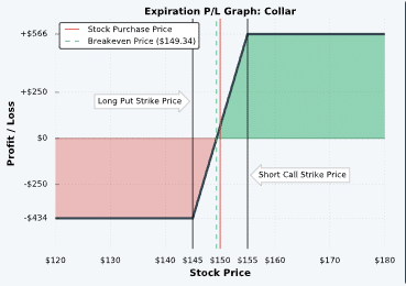
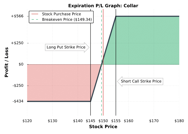
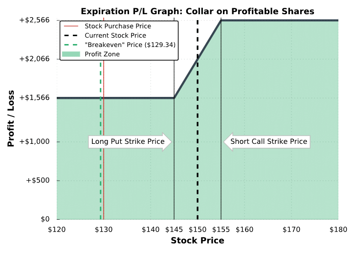
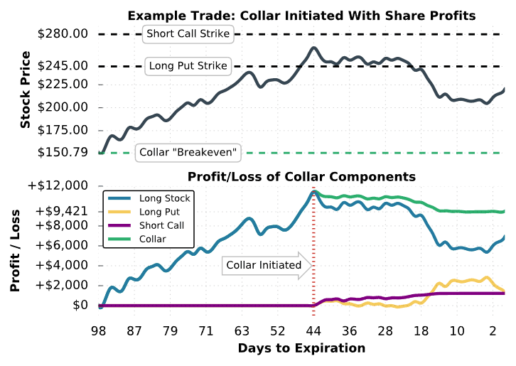
In the final example, we’ll examine how a collar position can be used to protect the profits on a long share position. Here’s the setup:

➥ Initial Share Purchase Price:$151.04

➥ Share Price When Entering Collar: $265.42

➥ Strikes and Expiration: Long 245 put; Short 280 call; Both options expiring in 44 days

➥ Premium Collected for Call: $12.30

➥ Premium Paid for Put:$12.05

➥Net Credit: $12.30 in premium collected – $12.05 in premium paid = $0.25 net credit

➥ Breakeven Price: $151.04 share purchase price – $0.25 collar credit = $150.79

➥ Maximum Profit Potential: 

[($280 short call strike – $151.04 share purchase price) + $0.25 collar credit] x 100 = +$12,921

➥ Maximum Loss Potential:*

[($245 long put strike – $151.04 share purchase price) + $0.25 collar credit] x 100 = +$9,421

*In this example, we’ve altered the maximum loss calculation to result in a positive number because this particular position has no loss potential. Using the standard formula from the other examples would give us a negative maximum loss number, which represents a profit. Adjusting the formula was done to avoid confusion.

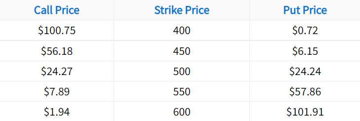
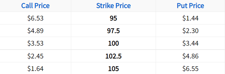
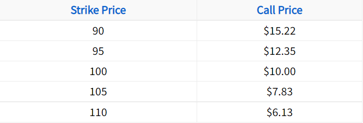
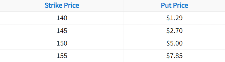
As we can see from the table above, there is no loss potential on this position because the share purchase price is well below the long put strike. Let’s see what happens over time:

Collar options strategy 2

Collar #3 Trade Results

As we can see from this scenario, the stock price did end up falling after the collar was entered. With the stock price below the long 245 put at expiration, the overall profit on the collar position was +$9,421 like we calculated previously. Meanwhile, the profit on the long stock position without the collar was +$7,500. The outperformance of the collar stems from the profits on both the long 245 put and short 280 call.

The example above demonstrates how collars are most commonly used in practice.

Final Word

Congratulations! You’ve learned the basics of how the collar strategy works, and how it’s commonly used in practice. In a nutshell:

  • Collars provide great downside protection in volatile markets.
  • Over the long run, outright stock tends to outperform collar trades.
  • If the premium collected from the call is equal to or greater than the premium paid for the put, the collar is said to be “cashless”.
Chris Butler portrait