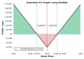
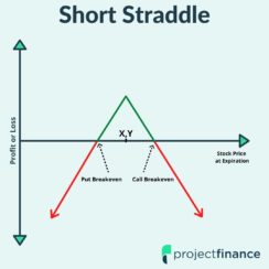
Options Trading Long Straddle Explained – The Ultimate Guide with Visuals Read More » February 10, 2022
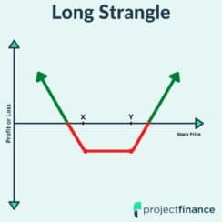
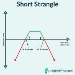
Options Trading Long Strangle Option Strategy with Visuals – The Ultimate Guide Read More » February 10, 2022
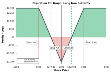
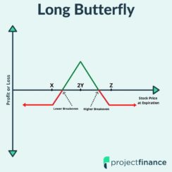
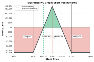
Options Trading Long Butterfly Spread Explained – Options Strategy with Visuals Read More » February 14, 2022