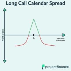
Options Trading How to Trade Options Calendar Spreads: (Visuals and Examples) Read More » February 28, 2022
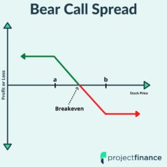
Options Trading Credit Spread Options Strategies (Visuals and Examples) Read More » February 28, 2022
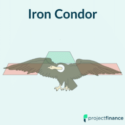
Options Trading Iron Condor Options Strategy (Visuals + Trade Examples) Read More » February 10, 2022