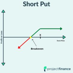
?> Chris Butler, Author at projectfinance - Page 3 of 10

Iron Condor Management Results from 71,417 Trades

Iron Condor Options Strategy

Selling iron condors is an extremely popular options strategy among income traders. In this guide, you’re going to see historical profitability results for the short iron condor strategy on the S&P 500 ETF.

Watch the video below for the key takeaways, or continue reading for all of the results.

Iron Condor Setups

While there are unlimited variations of the iron condor that we could test, we had to choose only a few, as the amount of data would be overwhelming for more than one or two variations. Here are the two iron condor variations that we’ll examine in this round of analysis:

1) 16-Delta Short Options & 5-Delta Long Options

2) 30-Delta Short Options & 16-Delta Long Options

By placing the short call and put at the 16-delta level, we sell “one standard deviation” options. By definition, one standard deviation encompasses 68% of outcomes around the average (the “average” being the current stock price, in this case).

As it relates to our short iron condors, selling one standard deviation options means we have an approximate 68% probability of the iron condor expiring worthless, which occurs when the stock price is in-between the short strikes at expiration.

In the case of the second iron condor setup, 30-delta options are at the half standard deviation level. Since the short strikes are much closer to the stock price, there’s a much lower probability that the iron condors expire worthless, since there’s a lower probability that the stock price is in-between the short strikes at expiration. Based on the call and put having an approximate 30% probability of expiring ITM, the estimated probability of these iron condors expiring worthless is about 40% (100% – 30% Call Prob. ITM – 30% Put Prob. ITM).

Iron Condor Management Combinations

For the sake of completeness, we’ll be testing 16 different iron condor management combinations for each short iron condor in this study:

1) Expiration (No Management)

2) Expiration OR -100% Loss

3) Expiration OR -200% Loss

4) Expiration OR -300% Loss

5) 25% Profit OR Expiration

6) 50% Profit OR Expiration

7) 75% Profit OR Expiration

8) 25% Profit OR -100% Loss

9) 50% Profit OR -100% Loss

10) 75% Profit OR -100% Loss

11) 25% Profit OR -200% Loss

12) 50% Profit OR -200% Loss

13) 75% Profit OR -200% Loss

14) 25% Profit OR -300% Loss

15) 50% Profit OR -300% Loss

16) 75% Profit OR -300% Loss

Each management level is based on the entry credit for the iron condors. For example, if an iron condor is sold for $1.00, a -200% loss would be when the loss is 200% of the entry credit, or $2.00. A loss of $2.00 would occur when the iron condor is worth $3.00 ($1.00 Entry + $2.00 Loss = $3.00).

Regarding profits, if an iron condor is sold for $1.00, a 75% profit occurs when the profit on the trade is $0.75, which occurs when the iron condor is worth $0.25 ($1.00 Entry – $0.75 Profit = $0.25).

By testing all of these iron condor management combinations, we can isolate performance changes by taking profits, taking losses, and the combination of the two.


Study Methodology: 16-Delta Iron Condors

Underlying: S&P 500 ETF (SPY)

Time Frame: January 2007 to March 2017

Entry Dates: Every trading day

Expiration Cycle: Standard expiration closest to 45 days to expiration (resulting in trades between 30-60 days to expiration).

Iron Condor #1: Sell the 16-delta call and 16-delta put. Buy the 5-delta call and 5-delta put.

Iron Condor #2: ​Sell the 30-delta call and 30-delta put. Buy the 16-delta call and 16-delta put.

Number of Contracts: 1

One important thing to mention is that these iron condors have more risk on the put side than the call side, as the downside volatility skew results in a wider put spread relative to the call spread.

For example, as I write this, the iron condor in SPY with the above setup is the 225/212 put spread ($13 wide) and the 243/247 call spread ($4 wide). In the future, we can test equal-width spreads.

Results: 16-Delta / 5-Delta Iron Condors

With 16 different management combinations, we’ve got a total of 40,868 iron condors included in the following results.

Let’s start with win rates.

Win Rates: 16-Delta / 5-Delta Iron Condors

Here are the percentages of profitable trades in each iron condor management approach:


Iron Condor Management: Percentage of Profitable Trades

As we would expect, the approaches with the highest success rates were the earlier profit-taking combinations. Additionally, the loss-taking approaches saw decreases in the rate of success, as more trades were closed for losses (some of which expired profitable).

However, win rates do not tell us the whole story. We can get a better idea of the most profitable approaches by comparing the realized success rate to the required breakeven success rate (based on the average profits and average losses for each approach).

Win Rates – Breakeven Rates

Here were the differences between the realized success rates and required breakeven success rates for each approach:


Iron Condor Management: Win Rates - Required Breakeven Win Rates

As we can see, even though the 25% profit approaches had the highest success rates, they outperformed their required success rates by the lowest margin compared to any other approach.

For example, in the 25% / Expiration management approach, if the success rate was 3.1% lower, the strategy would break even over time (based on the historical average profits and average losses). The higher the success rate is relative to the required breakeven success rate, the more positive the trade’s P/L expectancy will be.

Average P/L Per Trade

Let’s take a look at the average profit/loss per trade in each iron condor management approach:


Iron Condor Management: Average Profit/Loss

The lower profit percentage approaches saw a decrease in the average P/L per trade, which is what we’d expect when taking smaller profits while also allowing the same magnitude of drawdowns.

90th Percentile Losses

To compare the outlier drawdowns of each approach, we’ll examine the 90th percentile losses for each iron condor management combination. The 90th percentile loss tells us the loss level in which 90% of losing trades did not reach. In other words, only 10% of losses were worse than the 90th percentile loss.


SPY Iron Condors: Worst Losses

As expected, the tighter stop-loss approaches had the shallowest drawdowns of any approach. In regards to the profit or expiration approaches, the 25% management had the worst 90th percentile drawdown, which indicates of the few trades that were losers, the losses were typically substantial. Losses were consistent in the loss-taking approaches.

Average Time in Trades

Though some iron condor management approaches have substantially higher average profits per trade, not all trades are held for the same amount of time. So, we need to account for the fact that more trades can be squeezed into each 45-day period when closed earlier for profits or losses.

Let’s take a look at the average time in trades for each approach, and then normalize the average profit per trade of each approach to a 45-day period.

Here were the average number of calendar days held for the trades in each approach:


SPY Iron Condors: Average Time in Trade

As we’d expect, closing trades early for profits or losses results in less time in each trade. As a result, shorter average trade durations lead to more occurrences over time if a new trade is placed immediately after the previous one is closed.

Average P/L Per Trade (Adjusted for Time)

Let’s look at the average profitability of trades for each approach when normalized to a 45-day period. Here’s the calculation:

45-Day Adjusted Average P/L: Average P/L x (45 Days / Average Days in Trade)


SPY Iron Condors: Average Profit/Loss Adjusted for Time

When normalizing the average P/L per trade of each iron condor management approach, we find that there are many better alternatives to managing iron condors than simply holding to expiration (as the previous graphs may have suggested).

Based on these values, the 50-75% profit levels seem to stand out the most.

Commission Impact

Of course, we need to consider the commission impact of each approach. At this point, we’ve identified that the 45-day profit expectancy seems to be consistently high in the 50% and 75% profit-taking combinations. However, with more trade occurrences, commissions can become an issue, especially for an options strategy with four legs.

Let’s take a look at the 45-day expected commissions based on a $1 per contract commission schedule (no ticket/per-trade charge). Here’s the calculation for our commission estimations:

45-Day Commissions = (45 Days / Avg. Days Held) x $1 x 4 Contracts x 2 Trades (Open/Close)

= (45 Days / Avg. Days Held) x $8


SPY Iron Condor Commissions

As expected, the highest commissions occur in the lower profit/loss approaches, as those combinations generate the highest number of trades.

Average 45-Day P/L – 45-Day Commissions

Let’s look at the average 45-day P/L of each approach after taking out the estimated commissions over each 45-day period:


Iron Condor Commission-Adjusted Profit/Loss

Wow! Before adjusting for commissions, it seemed as if each approach had similar P/L expectancy. However, after taking out the estimated commissions over each 45-day period, it becomes clear that taking profits at 25% may not be the most efficient strategy.

Of course, these figures will vary depending on your particular commission rate, but a $1/contract commission structure with no ticket charge is on the lower end of available commission structures.

In the next section, we’ll examine the 30-delta short option and 16-delta long option iron condor variation.

Results: 30/16 Iron Condors (30-Delta Short, 16-Delta Long)

You’ll notice that we’ve omitted the -300% loss level for this particular iron condor setup. We did this because the spread widths are much narrower than the 16-delta short / 5-delta long iron condors. Only 2.5% of trades had loss potential greater than 300% of the credit received. However, 25% of trades had loss potential greater than 250% of the credit received, so we did include the -200% loss level.

Overall, having 12 iron condor management combinations gives us 30,549 trades.

Win Rates: 30-Delta / 16-Delta Iron Condors

Here were the percentages of profitable trades in each iron condor management approach:


SPY Iron Condors: Win Rate

Compared to the 16-delta short option and 5-delta long option iron condor setup, the 30-delta / 16-delta iron condors realized lower success rates across the board. However, the 25-50% profit percentage approaches still realized high success rates, despite the iron condors having an approximate 40% probability of expiring worthless.

Let’s see how these win rates stacked up against the required breakeven win rates calculated from the average profits and average losses for each approach.

Win Rates – Breakeven Win Rates

Here are the differences between the realized success rates and required breakeven success rates for each approach:


SPY Iron Condors: Win Rates - Breakeven Success Rates

Completely opposite of the 16-delta iron condors, the 25% profit percentage approaches for the 30-delta iron condors saw the highest margins over the required breakeven success rates. Conversely, the higher profit percentage approaches exceeded the required breakeven win rates by very thin margins.

The data suggests that when the short options are closer to the stock price (closer to ±0.50 delta), closing profitable trades early has been more favorable than closing at higher profit percentages.

Average P/L Per Trade

Let’s take a look at the average profit/loss per trade in each iron condor management approach:


SPY Iron Condors: Average Profit/Loss

As the Win Rate – Required Breakeven Win Rates would suggest, the 25-50% profit percentage approaches saw the highest average P/L per trade. Interestingly, the -200% loss category experienced higher average P/L than the no-loss approaches. This can be explained by the fact that -200% is near max loss for most of these iron condors. While locking in the maximum loss on a limited-risk spread isn’t very logical in practice, it’s still interesting to see that taking losses slightly lower than the maximum loss enhanced average profitability over the long-term.

90th Percentile Losses

To compare the largest drawdowns of each approach, we’ll examine the 90th percentile losses for each iron condor management combination. The 90th percentile loss tells us the loss level in which 90% of losing trades did not reach. In other words, only 10% of losses were worse than the 90th percentile loss.


SPY Iron Condors: Worst Drawdowns

As expected, the tighter stop-loss approaches had the shallowest drawdowns of any approach. The -200% loss combinations saw drawdowns very close to the no stop-loss approach of holding trades to expiration, which suggests the trades were closed without much more loss potential (not the most logical approach, but included nonetheless).

Average Time in Trade

As we did before, let’s examine the average time in trades for each approach, and then normalize the average profit per trade of each approach to a 45-day period.

Here were the average number of calendar days held for the trades in each iron condor management approach:


SPY Iron Condors: Average Time in Trade

As we’d expect, closing trades early for profits or losses results in less time in each trade. As a result, shorter average trade durations lead to more occurrences over time if a new trade is placed immediately after the previous one is closed.

Average P/L Per Trade (Adjusted for Time)

Let’s look at the average profitability of trades for each approach when normalized to a 45-day period. Here’s the calculation for reference:

45-Day Adjusted Average P/L: Average P/L x (45 Days / Average Days in Trade)


Iron Condors: Average P/L Per Trade

When normalizing the average P/L per trade of each iron condor management approach, the 25% profit levels were the clear winners, with the 50% profit levels following close behind. But, as we know, we need to see the percentage of profits given back to commissions before determining the “optimal” management approaches.

Commission Impact

Like we did for the previous iron condor variation, let’s look at the 45-day avg. P/L when adjusted for commissions. Estimated commissions are based on a $1 per contract commission schedule (no ticket/per-trade charge).

First, here are the estimated 45-day commissions for each approach:


SPY Iron Condors: Commission Impact

Consistent with the findings from the 16-delta iron condors, closing trades earlier (for a profit or loss) generates more overall occurrences in the same period of time. As a result, the commissions were the highest in the 25-50% profit percentage approaches.

Now let’s subtract these commissions from the 45-day P/L expectancy for each approach:


SPY Iron Condors: Commission Adjusted P/L

Opposite of the 16-delta iron condors, the 25-50% profit target combinations had the highest P/L expectancy when adjusted for commissions.

Iron Condor Performance by VIX Level

Now that we’ve examined the performance of two iron condor variations with 16 different management combinations, let’s filter the trades into four VIX buckets with an equal number of trades. To accomplish this, we’ll use the 25th, 50th, and 75th percentile of VIX levels over the test period to evenly divide the trades into four volatility buckets.

Here are the four VIX ranges for each bucket:

Low: VIX Below 14

Low-Mid: VIX Between 14 and 17.5

Mid-High: VIX Between 17.5 and 23.5

High: VIX Above 23.5

16-Delta Iron Condors vs. VIX at Entry

Let’s start with success rates:


SPY Iron Condors vs. VIX

The results show consistently higher success rates in trades entered when the VIX was below 17.5, with some management combinations realizing a spike in success rates when trades were entered in high implied volatility environments.

How do these success rates stack up against the required breakeven success rates (based on average profits and average losses)?

Win Rates – Breakeven Win Rates

Here’s the difference between the realized success rates and required breakeven success rates for each approach:


Iron Condor Management: Win Rates - Required Breakeven Win Rates

In the approaches that did not take losses, the highest margins of success rates over the breakeven success rates occurred in the low IV entries. The approaches that took losses with high profit targets exceeded the required breakeven success rate by the largest margin in the high IV entries.

The findings suggest that when iron condors are sold in high IV environments, the losses tend to be substantial relative to the profits (especially when closing profits early). By taking early losses on losing trades in high IV environments, the losses are kept manageable, while profitable trades drive solid returns on a per-trade basis.

In the next section, we’ll look at profit metrics for the trades in each volatility environment.

Average Profit/Loss Per Trade

Here were the average P/L figures for the iron condors in each approach:


Iron Condor Management: Average Profit/Loss

The average P/L metrics tell us that managing losing trades in high IV environments substantially increased the overall profitability of trades, as losses were kept small while profitable trades enjoyed heightened gains. 

Additionally, closing profitable trades at lower profit percentages in high IV environments had the worst performance, as profitable trades were cut short while losses were still substantial. The combination of these two things results in a high required win rate to break even, which makes it harder to profit over the long-term.

90th Percentile Losses

To validate previous statements, we’ll examine the 90th percentile losses for the iron condors in each volatility environment. The 90th percentile loss indicates the level that only 10% of trades exceeded. In other words, the 90th percentile loss is rare.


As we can see, the high IV entries saw the worst drawdowns in every single management approach. These loss figures help explain why taking losses in the higher IV entries substantially improved overall profitability per trade.

Average Time in Trade

Here’s the average number of calendar days held for the trades in each approach:


As we’d expect, closing trades early for profits or losses results in less time in each trade.

Average P/L Per Trade (Adjusted for Time)

Let’s look at the average profitability of trades for each approach when normalized to a 45-day period. Here’s the calculation:

45-Day Adjusted Average P/L: Average P/L x (45 Days / Average Days in Trade)


In low volatility environments, closing profitable trades early generated the highest average profitability over 45-day periods. The high IV entries saw the most profitability over 45-day periods in each loss-taking approach. This makes sense, as we know that the largest losses occurred during the high IV entries.

In the final section, we’ll examine how much commissions reduced the performance of each approach.

45-Day Average Profitability (Adjusted for Commissions)

Let’s take a look at the 45-day average P/L of each approach when adjusted for commissions over the same period. Commissions are based on a $1 per contract commission schedule. Here’s the calculation for the adjusted average profitability:

Number of Trades: (45 Days / Avg. Days Held)

Commissions Per Trade: 4 Options x $1 x 2 Transactions (Open/Close) = $8

45-Day Adjusted P/L: 45-Day Avg. P/L – (Commissions Per Trade x Number of Trades)


As we can see here, there are a few approaches with negative P/L expectancy when adjusting for commissions. All of the negative P/L approaches included taking profits at 25% of the maximum profit potential.

The highest P/L expectancies occurred in the loss-taking approaches when entered in high implied volatility environments.

As mentioned earlier, these figures will vary depending on your particular commission rate.

30-Delta Iron Condors vs. VIX at Entry

We’ll finish with the same analysis applied to the 30-delta short option / 16-delta long option iron condor variation!

Let’s start with success rates:


Iron Condor Management: Percentage of Profitable Trades

With the short options being much closer to the stock price at entry, closing profitable trades early significantly improved win rates. Furthermore, the larger stop-loss and expiration approaches saw the highest win rates in the lowest and highest VIX entries.

Win Rates – Breakeven Win Rates

Here were the differences between the realized success rates and required breakeven success rates for each approach:


Iron Condor Management: Win Rates - Required Breakeven Win Rates

Interestingly, most of the approaches that did not close profitable trades early realized win rates less than the required win rates to break even in the mid-level VIX entries.

The trades with the highest success rates relative to the required breakeven success rates were the high VIX entries, suggesting that selling options closer to the stock price has been beneficial in high volatility environments.

Average P/L Per Trade

Here were the average P/L figures for the iron condors in each approach:


Iron Condor Management: Average Profit/Loss

Consistent with the positive Win Rate – Breakeven Success Rate approaches, the iron condor management combinations with the highest average P/L per trade were the high VIX entries.

90th Percentile Losses

How large were the losses in each volatility environment? Here were the 90th percentile losses for each approach:


Similar to the 16-delta iron condors, the largest losses were in the high VIX entries. However, there was less dispersion between losses in each volatility environment, which likely stems from the fact that the 30-delta iron condors have less overall risk relative to the potential reward.

Average Time in Trade

Here’s the average number of calendar days held for the trades in each approach:


As we’d expect, closing trades early for profits or losses results in less time in each trade.

Average P/L Per Trade (Adjusted for Time)

Let’s look at the average profitability of trades for each approach when normalized to a 45-day period. Here’s the calculation:

45-Day Adjusted Average P/L: Average P/L x (45 Days / Average Days in Trade)


By analyzing the 45-day adjusted average P/L for each approach, it becomes very clear that the 30-delta iron condor variation has historically performed very well in high implied volatility environments. 

45-Day Average Profitability (Adjusted for Commissions)

Let’s take a look at the 45-day average P/L of each approach when adjusted for commissions over the same period. Commissions are based on a $1 per contract commission schedule. Here’s the calculation for the adjusted average profitability:

Number of Trades: (45 Days / Avg. Days Held)

Commissions Per Trade: 4 Options x $1 x 2 Transactions (Open/Close) = $8

45-Day Adjusted P/L: 45-Day Avg. P/L – (Commissions Per Trade x Number of Trades)


Consistent with previous statements, the high VIX entries were the clear winners in regards to the 30-delta iron condor variation.

Summary

We’ve just made it through a ton of data, so let’s quickly recap the most notable findings from this study!

Iron Condor Variation #1: 16-Delta Short Options & 5-Delta Long Options

In regards to the 16-delta iron condors, each approach appeared to have similar P/L expectancy when accounting for the number of trades that could be squeezed into a 45-day period. However, when adjusted for estimated commissions, the 50-75% profit target approaches stood out the most in terms of P/L expectancy:


When closing profitable trades for 50-75%, the number of overall trades increases since positions are closed faster. This allows traders to “re-center” their iron condor trades sooner, and position themselves in the next expiration cycle. However, the 50-75% profit target combinations do not churn trades as often as the 25% profit target approaches, which results in less commissions and higher expectancy over time.

Implied Volatility & Performance: 16-Delta Short Options & 5-Delta Long Options

When filtering for VIX levels at trade entry, the trades with the highest commission-adjusted P/L expectancy were the loss-management and high profit target combinations with high VIX entries:


Iron Condor Variation #2: 30-Delta Short Options & 16-Delta Long Options

Unlike the 16-delta iron condors, the 30-delta iron condors saw the highest commission-adjusted P/L in the 25-50% profit target approaches. Since the short options are much closer to the stock price, the trades need to be held for much longer to achieve the 75-100% profit levels. Historically, waiting for these profit levels has not been favorable (without filtering for IV at entries).


Implied Volatility & Performance: 30-Delta Short Options & 16-Delta Long Options

After filtering for VIX levels at the entries of all trades, we found that the 30-delta iron condors have historically performed the best when entered in high VIX environments:


No matter the management combination, entering these tighter iron condor trades in high volatility environments has resulted in the most efficient trades in terms of commission- and time-adjusted P/L.

Hopefully, this in-depth study can help guide you towards more informed trading decisions when trading iron condors in equity indices.

Thank you for reading!

Next Lesson

Additional Resources

Iron Condor FAQs

When sold sufficiently out of the money, iron condors have a success rate greater than 50%. However, selling out of the money iron condors comes with greater risk and less profit potential than iron condors sold closer to being in the money. 

On the short iron condor strategy, the maximum loss is limited to the difference between the strike prices of either spread, multiplied by the contract size, minus the premium received.

Since the iron condor has defined risk, this options strategy is relatively save when compared to strategies such as the short call and short put. 

Chris Butler portrait

Here’s How Scalping in Trading Works

If you’ve been listening to traders talk on the news, podcasts, or educational videos, you may have heard them use the term “scalping.” So, what is scalping?

Scalping Explained

Scalping refers to an activity where traders try to buy or sell securities (stocks, options, or futures contracts) for short-term gains. For example, most long-term investors will buy stocks in their investment portfolios and hold those stocks for many years before selling them.

Let’s look at an example with Apple (AAPL):


Long-Term Investment Example

In the case of a normal investor, the investment/trade time frame is typically many years.

When scalping, the duration of each trade could be as little as a few minutes to a few hours. Generally speaking, scalping is an “intraday trading” activity, which simply means all of the trades are opened and closed within the trading session. Here’s an example of scalping AAPL stock:


What is Scalping? AAPL Scalping Example

In this case, we can see AAPL’s price fluctuations over one trading day (each bar is a 5-minute period). A scalper will try to predict AAPL’s short-term movements to extract profits over time.

What Can Traders Scalp?

In the trading world, any product can be scalped. There are traders who primarily scalp shares of stock, while others may scalp options or futures contracts.

All in all, “scalping” refers to trading over short time frames.

Can You Make Money Scalping?

While the idea of trading short-term fluctuations in stocks, options or futures is enticing, keep in mind that transaction costs are higher for more active, short-term trading.

Additionally, it’s very difficult, if not impossible, to predict stock price movements. So, the profitability of a scalping trading approach will come down to having a solid system that a trader can follow. The system should aim to keep drawdowns small (get out of losing trades when you’ve been proven wrong), and maximize winning trades.

For example, if a scalpers trading system has a 1:3 risk/reward relationship, the trader only has to have a success rate of 25% (since one winning trade evens out three losing trades) to break even. So, if the trader can pick entries that result in a success rate higher than 25%, the strategy will be profitable over time.

At projectoption, we do not scalp in our live trading portfolio, as we typically trade options with 30-60 days to expiration.

Chris Butler portrait

What is Option Buying Power? | Options Trading Concept

Option Buying Power Definition: The total amount of funds currently available to trade options with. 

When trading stocks, options, or futures, you have to have the appropriate amount of cash available in your account to open a position.

The term “Buying Power” refers to the amount of money in your account that is readily available to allocate to new positions.

Stock buying power and option buying power differ, so let’s start with stock buying power.

Stock Buying Power

Stock Buying Power Definition: Total amount of money available to trade stock with. Equals available cash + available margin. 

Depending on the type of account you have, your stock and option buying power may differ. For margin accounts, the margin requirements to trade stock is less than that of options. 

If you have a standard margin account, your stock buying power will typically be 2x the amount of cash you have available in your account, as margin accounts have the ability to buy shares of stock with 50% of the position’s notional value (resulting in 2:1 leverage).

As an example, if you want to buy 100 shares of a $200 stock, the notional value is $20,000 ($200 per share x 100 shares = $20,000 value). In a cash account, you’d need $20,000 of available buying power to purchase those shares. 

However, in a margin account with 2:1 margin capabilities, you’d only need $10,000 of available stock buying power to purchase $20,000 worth of stocks.

Here’s a table that quickly demonstrates the required stock buying power for certain stock purchases based on the account type:

buying power

In some margin trading accounts, the stock buying power can reach 4x the available cash in the account for intraday stock trading. As a result, traders can reach 4:1 leverage for stock trades that are opened and closed within a single trading day.

Care to watch the video instead? Check it out below!

Option Buying Power

Unlike stock buying power, options cannot be purchased on margin. As a result, option buying power is equal to the amount of cash in your account that is readily available to allocate to option positions.

For example, let’s look at the “buying power effect” of buying to open an AAPL call option that’s trading for $5.75:

Software Used: tastyworks Trading Platform

As we can see, the buying power effect is “reduced by $576.14”, which means purchasing the AAPL call option for $5.75 reduces our available buying power by $576.14.

Why $576.14? Well, a $5.75 equity option is worth $575 in dollar terms ($5.75 Option Price x Standard Option Contract Multiplier of 100 = $575). The additional $1.14 in this case comes from the commission cost of entering the position.

When you purchase an option, the most you can lose is the value of that option (Option Price x Option Contract Multiplier). So, you’ll always have to have enough cash in your account to cover the entire cost of an option position.

The same is true for option spreads you purchase. Here’s an AAPL put debit spread:

Software Used: tastyworks Trading Platform

The net cost of the spread is $2.63 ($263 in actual value), plus $2.29 in commissions. As a result, $265.29 in option buying power is required to purchase this put spread.

Option Buying Power Required to Sell Spreads

You know that to buy an option you need to have enough available cash in your account to cover the maximum loss and commissions associated with an option purchase. How much do you need in your account to sell options?

When it comes to limited risk spreads, you’ll need option buying power equal to the maximum loss of the spread, plus commissions. Here’s an example of the buying power required to sell a put spread in NFLX:

(Hint! Click to enlarge)

Software Used: tastyworks Trading Platform

In this example, we’re selling a $10-wide put spread for $3.41, which means the maximum loss on the spread is $659 ($3.41 Entry Credit – $10 Maximum Spread Value = -$6.59 x 100 = -$659). With $2.30 in commission costs, we’d need $661.30 in option buying power to sell this put spread.

Pretty simple!

Option Buying Power: Selling Naked Options

What about option positions with “unlimited” loss potential?

For option positions with substantial loss potential (short callsshort puts), the buying power requirement is commonly calculated as the greatest value of three calculations:

Calculation #1: 20% of the current stock price – the out-of-the-money amount + current value of the short option.

Calculation #2 (Call Options): 10% of the stock price + current value of call option.

Calculation #2 (Put Options): 10% of the strike price + current value of put option.

Calculation #3: $50 per option contract + current value of option.

As an example, here’s the estimated option buying power requirement for a put option on a $100 stock

*[($100 x 20%) – $10 OTM + $2.50]  x 100

**[($90 x 10%) + $2.50] x 100

***$50 + ($2.50 x 100)

Based on the three margin values from the calculations, you would need $1,250 in option buying power to sell this particular put option.

Fortunately, you won’t have to ever make these calculations, as your brokerage firm will take care of the calculations for you!

Changes in Buying Power

For limited risk option positions (such as option spreads or outright option purchases), your buying power requirement will not change over the duration of the trade because the risk is always known.

However, for uncovered option positions (short calls and short puts), the buying power requirement will change as the stock price, option premium, and out-of-the-money amount change. As a result, it’s always a good idea to never “max out” your account’s option buying power, as an increase in the buying power requirement can lead to your brokerage firm forcing you out of positions if you can no longer meet the capital requirement.

Hopefully, this post has helped you learn about the required costs associated with opening new stock and option positions in your trading account (non-margin cash or regular margin).

Option Buying Power FAQs

In options trading, the buying power effect represents a transactions net effect on the future available funds to trade options. When you buy options, a debit is taken from your account (like stock). When you sell options, buying power is reduced because of the margin required to hold the trade.

Negative buying power implies you do not have adequate on-hand cash to hold all positions in your account. This may be indicative of a margin call. Best practice is to make cash available, or call your broker if the buying power calculation is faulty.  

Stock typically takes 2 business days to settle; options usually take one business day to settle. After this time period, your buying power should free up.

Chris Butler portrait

Moneyness of an Option Explained | What You Need to Know

option moneyness chart calls and puts

Options traders often use “moneyness” to describe the relationship between an option’s strike price and the current stock price. Here’s how it works. 

What is Option Moneyness?

The moneyness of an option refers to three specific options trading terms:

1. In-the-Money

2. At-the-money

3. Out-of-the-money​

Let’s quickly discuss each of these terms in regards to call and put options.

What is an “In-the-Money” Option?

An “in-the-money” option is any option contract that currently has intrinsic value. If you’re unfamiliar with intrinsic and extrinsic value, intrinsic value simply means that the option will be worth something at expiration if the stock price remains at its current level. Let’s take a look at some examples:

As we can see here, call options are “in-the-money” when the call’s strike price is below the current stock price, as that means the call has intrinsic value.

The opposite is true for put options:

As the table suggests, any put option with a strike price above the current stock price is considered in-the-money, as the put option has intrinsic value.

Here’s a picture showing the in-the-money options for IWM when the stock is trading for $137.21:


Moneyness of an option: In-the-Money

What is an “At-the-Money” Option?

The moneyness of an option is said to be “at-the-money” when the option’s strike price is very close or equal to the current stock price. The concept applies to both call and put options.

Here’s a visual showing the real at-the-money options in IWM with the stock trading at $137.21:

Moneyness of an option: At-the-Money

While the 137 call option is technically in-the-money since its strike price is below the stock price, the 137 call would be the call option that’s considered at-the-money.


What is an “Out-of-the-Money” Option?

Lastly, the moneyness of an option is said to be “out-of-the-money” when the option has no intrinsic value. That means a call option is out-of-the-money when the strike price is above the stock price:


Here’s a snapshot of all the out-of-the-money options with IWM trading at $137.21:


Moneyness of an option: Out-of-the-Money

Here’s a snapshot of all the out-of-the-money options with IWM trading at $137.21:

Congratulations! You now know what the moneyness of an option is! Now, you’ll always know what an options trader is talking about when they use the moneyness terms to describe an option.

Chris Butler portrait

Iron Condor Options Adjustment: Rolling the Short Call

Iron Condor Options Strategy

Sometimes, you’ll need to make an adjustment to your option positions when the stock price moves against you.

In this post, you’ll learn about the iron condor adjustment of “rolling down” the short call spread to defend an iron condor.

What You’ll Learn

1. What “rolling down” a short call spread means.

2. How rolling down the short call spread can minimize risk and maximize profits in a troubled iron condor position.

3. The one drawback of rolling down the short call spread to defend the trade.

Let’s get started!

What is “Rolling?”

In options trading, “rolling” refers to closing an existing option position and opening a similar option position with different strike prices, in a different expiration cycle, or a combination of the two.

Today, we’ll focus on “rolling down” the short call spread in a short iron condor position, which refers to buying back your current call spread and “rolling it down” by selling a new call spread at lower strike prices.

Rolling an Option

The process of closing an existing option and opening a similar option position at different strike prices, in a different expiration cycle, or a combination of the two.

When Do You Roll Down the Short Call Spread?

When trading iron condors, the most typical time to roll down the short call spread is when the stock price falls quickly towards your bull put spread.

Consider the following visual:


Iron Condor Adjustment: Rolling Down the Short Call Spread

Typically, a short iron condor position will start with no directional risk exposure (position delta is near zero). However, when the stock price falls quickly towards the short put’s strike price, the position’s delta will grow positive, which means the trade has become directionally bullish.

The most common iron condor adjustment to make in this scenario is to roll down the short call spread by purchasing the old call spread (closing trade), and selling a new call spread at lower strike prices (opening trade):


Iron Condor Adjustment: Rolling Down the Short Call Spread

When adjusting an iron condor by rolling down the short call spread, what does the trader accomplish?

What Does Rolling Down the Call Spreads Accomplish?

By rolling down the call spread to lower strike prices, a trader accomplishes two things:

1. Collect More Option Premium

Since call options at higher strike prices are cheaper than call options at lower strike prices, rolling down the old short call spread to lower strike prices is done for a net credit. “Net credit” just means more option premium is collected than paid out.

By collecting more option premium, the iron condor position’s maximum loss decreases by the amount of premium received (assuming the spread widths remain the same). For example, if a $5-wide iron condor is initially sold for $1.00 and the trader rolls down the call spreads for a $0.50 credit, the position’s maximum loss decreases by $0.50 and the maximum profit increases by $0.50. 

However, the put spread and call spread are now closer together, which means the iron condor position has a narrower range of maximum profitability.

2. Neutralize Directional Exposure

By rolling down the call spreads, the iron condor’s directional exposure shifts from bullish to closer to neutral.

Why?

At the time of rolling down the call spreads, an iron condor will have a positive position delta, which means the trader will lose money from subsequent decreases in the stock price.

When the call spreads are rolled down to lower strike prices, the new short call spread’s delta will be more negative than the old short call spread, which reduces the iron condor’s position delta.

Let’s cover each of these points in more depth.

#1 Collect More Premium

Consider a trader who is short the 160/165 call spread in their iron condor position but rolls down to the 150/155 call spread:

How much option premium is collected from the roll?

Premium Collected:

$1.82 Collected from 150/155 Call Spread

– $0.53 Paid for the 160/165 Call Spread

+$1.29 ($129 Less Risk & $129 More Profit Potential)

By rolling down the short call spread, the trader collects $1.29 in additional option premium. With $1.29 more option premium collected, the iron condor has $129 more profit potential and $129 less loss potential.

However, since the new call spread is now closer to the put spread, the position has a much more narrow range of maximum profitability, which makes it a lower probability trade.

#2: Neutralize Your Position Delta

At the time of the roll, let’s say the trader’s position delta is +20. Here’s how the position delta would change after the roll:

Let’s break down the differences in each call spread’s delta and see how the new call spread changes the iron condor’s directional exposure:

Short 160/165 Call Spread Delta: -8 (-17 Delta Short Call + 9 Delta Long Call)

Short 150/155 Call Spread Delta: -17 (-47 Delta Short Call + 30 Delta Long Call)

Change in Call Spread Deltas: -9

New Iron Condor Delta: +20 – 9 = +11

To clarify, the call spread deltas are calculated with the following formula:

(Short Call Delta x -1 Contract x 100 Option Multiplier) + (Long Call Delta x +1 Contract x 100 Option Multiplier)

After rolling down the call spread, the iron condor’s delta exposure changes from +20 to +11, which means the iron condor is now 45% less sensitive to small changes in the stock price.

More specifically, the trader is only expected to lose $1 with a $1 decrease in the stock price as opposed to a $20 loss before the iron condor adjustment.

What’s the Risk of Rolling Down the Call Spreads?

While rolling down the short call spread has its benefits (higher maximum profit potential, lower loss potential, reduced directional exposure), there are some downsides:

1. Narrower Range of Profitability

An iron condor’s maximum profit zone lies between the short call and short put strike price. After rolling down the call spreads, the short call and short put strike prices are now much closer, which results in a much narrower range of maximum profitability.


2. Neutralized Directional Exposure

By neutralizing the iron condor’s directional exposure, a subsequent rally in the stock price will yield less profits (or even losses) than before rolling down the call spreads.

As with any trade adjustment, there are benefits and downsides. The iron condor adjustment strategy of rolling down the short call spreads decreases the loss potential, increases the profit potential, but ultimately makes the trade a lower probability position since the maximum profit zone is now tighter.

Concept Checks

Here are the essential points to remember the iron condor adjustment of rolling down the short call spreads:


1.When selling iron condors, if the share price falls towards your short put spread, you can adjust the position by “rolling down” the short call spreads.


2. By rolling down the old call spreads, you collect more option premium, which increases the maximum profit potential and decreases the maximum loss potential.


3. The downside of rolling down is that you decrease your probability of making money (tighter range of profitability), and make less money (or potentially lose money) from subsequent increases in the stock price.

Chris Butler portrait

Short Put Option Payoff Results from 41,600 Trades [Study]

Short Put Option Graph

The short put option strategy is popular among optimistic investors and traders who have a bullish outlook for a stock but don’t mind buying shares if the stock price falls.

In this post, we’ll examine over 10 years of 16-delta short put management data from 41,600 trades in the S&P 500 ETF (SPY).

More specifically, we’ll answer the following questions:

1. Which strategies were the most profitable?

2. Which strategies were the least profitable?

3. How did implied volatility at the time of entering the trade impact the overall profitability?

Stick around!

I guarantee you will learn something valuable that you can start incorporating in your trading today.

Study Methodology

Underlying: S&P 500 ETF (SPY).

Time Frame: January 2007 to May 2017 (most recent standard expiration, as of this writing).

Entry DatesEvery Trading Day.

Expiration CycleStandard Expiration Closest to 45 Days to Expiration (resulted in trades between 30-60 days to expiration).

TradeSell the 16-Delta Put Option

Number of Contracts1

Short Put Trade Management

For each entry, we tested 16 different management combinations:

Profit or Expiration: 25% Profit, 50% Profit, 75% Profit, OR Expiration.

Profit or -100% Loss: 25% Profit, 50% Profit, 75% Profit, OR -100% Loss.

Profit or -200% Loss: 25% Profit, 50% Profit, 75% Profit, OR -200% Loss.

Profit or -300% Loss: 25% Profit, 50% Profit, 75% Profit, OR -300% Loss.

Management Example: 50% Profit or -200% Loss

To demonstrate how we calculated the profit and loss levels, let’s run through a quick example using a 50% profit OR -200% loss target.

Entry Credit: $1.00

Profit Target: $0.50 ($1.00 Entry Credit – $1.00 x 50%)

Loss Limit: $2.00 ($1.00 Entry Credit x 200%). A $2.00 loss would occur when the put option traded $3.00 ($1.00 Entry Credit + $2.00 Loss).

Metrics We’ll Analyze

Before we get started, I want to quickly cover the primary metrics we’ll analyze:

Win Rates: The percentage of trades that were profitable.

Win Rate – Breakeven Win Rate: The difference between the success rate and what the strategy required to break even (based on average profits and losses). 

Average P/L: The average profitability of each trade. The average P/L figures will be consistent with the Win Rate – Breakeven Win Rate levels.

10th Percentile P/L: The P/L that 90% of trades exceeded (a probabilistic way of analyzing the worst drawdowns).

45-Day Adjusted P/L: Not all trades were held for the same amount of time. We standardized the average P/L of each trade to a 45-day period.

Win Rates: 16-Delta Short Puts

As expected, closing profitable trades early boosted the success rate, while taking losses reduced the success rate:

SPY Short Put Success Rates

Before moving on, I want to clarify the x-axis labels on the charts.

As an example, “25% / Exp.” means the trades were closed for 25% of the maximum profit potential OR held to expiration.

“Exp. / -200%” means the trades were held to expiration OR closed for a -200% loss.

Win Rates – Breakeven Win Rates

One of the more interesting metrics we analyze is the win rate minus the breakeven win rate, or the win rate that’s required for the strategy to break even over time. The breakeven win rate is calculated using the average profit and average loss of all the trades.

In a coin-flipping contest, if you win $1 for each toss that lands on heads and lose $1 for each toss that lands on tails, you’d need a 50% win rate to break even over time.

However, if you’re somehow able to win 60% of the time, then your Win Rate – Breakeven Win Rate would be 10% (60% Success Rate – 50% Breakeven Win Rate), and you’d make money over time.

Let’s take a look at the Win Rate – Breakeven Win Rate statistics for the short put trades:

SPY Short Put Breakeven Win Rates

Right out of the gates, we can see that the quicker profit-taking management combinations had the lowest margin between the success rates and the breakeven success rates, even though they had the highest success rates.

What does this mean?

Well, the 25% Profit / Exp. combination had a 98% success rate overall, but with a 2.2% Win Rate – Breakeven Win Rate, the strategy required a 95.8% success rate just to break even over time (based on the average profit of winning trades and the average loss of losing trades).

As it relates to your trading, just know that if you take profits very quickly, you will need a higher success rate over time to break even (since profits are so small relative to potential losses). For some, that may be daunting, and therefore may be better suited with a larger profit management strategy.

Average P/L Per Trade

Which short put management strategies were the most profitable, on average?

Short Put Strategy Average P/L

Since 2007, doing nothing and simply holding short put positions (16-delta, 30-60 DTE) to expiration has resulted in the highest average P/L per trade.

Consistent with the Win Rate – Breakeven Win Rates, the smaller profit-taking approaches had the lowest average profitability, which makes sense because the profits are taken much quicker and do not absorb losing trades as easily.

These figures are telling by themselves, but we don’t have the whole story. Let’s take a look at the worst drawdowns of each approach.

10th Percentile P/L

If you recall, the 10th percentile P/L tells us the P/L level that 90% of trades exceeded. For example, if the 10th percentile P/L is -$1,000, then 90% of trades had a P/L better than a loss of $1,000.

Let’s take a look at these “worst-case” drawdowns for each approach:

SPY Short Put Drawdowns

While the “do nothing” approach to selling puts has historically yielded the highest average P/L per trade, the “worst-case” drawdowns were also substantial. So, before jumping straight into the strategy with the highest average P/L, consider the drawdowns of that particular strategy.

As expected, the loss-taking approaches had substantially lower drawdowns. 

When considering the average P/L per trade and the 10th percentile P/L metrics together, the loss-taking approaches become considerably more attractive.

At this point, we’ve uncovered an astonishing amount of information related to S&P 500 put-selling strategies.

But we’re not done yet.

In the next section, we’ll analyze the average time in trades for each approach, and then adjust the average P/L per trade of each approach to a 45-day period.

Average Time in Trade

Let’s first start with the average time in each trade for all of the approaches:

As we’d expect, incorporating some type of profit or loss management results in fewer days in each trade, on average. How does the reduced time in each trade impact the hypothetical average P/L over similar time periods?

To answer this question, we’ll normalize the average P/L per trade of each approach to a 45-day period:

45-Day Adjusted Average P/L = Avg. P/L Per Trade x (45 / Avg. Days in Trade)

Of course, this isn’t a perfect formula, but it does help put context around the “average profitability” of each approach based on the number of trades that can “fit” into similar periods of time.

After normalizing each short put management approach’s expectancy to a 45-day period, we find that the smaller profit-taking approaches yield the highest P/L figures because trades are closed and redeployed much faster.

However, keep in mind that opening and closing trades more often will generate more commission costs.

Additionally, by closing a profitable short put and selling a new short put, the strike price will likely be higher and your delta (directional) exposure will be more positive. The result is more severe drawdown potential if the market corrects after the new trade is opened.

Short Put Performance by VIX Level

The analysis in this post would not be complete without some implied volatility filtering. In the case of the S&P 500, the implied volatility levels can be gauged by the VIX Index.

In this final section, we’ll analyze some of the metrics from above, but we’ll evenly divide all of the trades into four buckets based on the VIX level at the time of entering the trades:

1. VIX Below 14

2. VIX Between 14 and 17.5

3. VIX Between 17.5 and 23.5

4. VIX Above 23.5

These VIX levels were selected based on the 25th, 50th, and 75th percentile of VIX levels at the time of all trade entries. By using these percentiles, we evenly divide all trades into four separate buckets and avoid any one bucket having substantially more or less occurrences than the rest.

The next sections hold some of the most interesting takeaways from this entire post, so be sure you keep reading.

Short Put Win Rates by VIX Level

When analyzing the win rates of each approach based on the VIX at entry, there weren’t any screaming takeaways:

However, things start to get very interesting when we dive a bit deeper.

Win Rates – Breakeven Win Rates by VIX Level

When we look at the difference between success rates and what was required to break even (based on average profits and average losses), we see that the passive approaches had the most “edge” in the lower VIX environments:

In the higher VIX environments, the loss-taking approaches significantly outperformed the profit-or-expiration approaches. We’ll see this relationship carry over to the average P/L per trade.

Short Put Average P/L by VIX Level

Let’s take a look at the average P/L per trade based on the VIX levels at entry:


These results are fascinating, as they show that more passive approaches (taking larger profits and not taking any losses) performed the best in the lower VIX environments.

However, the approaches with higher profit targets that also included a loss-taking strategy performed the best in the highest VIX environments.

The results suggest that during more volatile market periods, it has been wise to let profitable trades run while aggressively closing losing trades.

10th Percentile P/L by VIX Level

To fully understand the previous results, let’s look at the worst-case drawdowns of each approach based on the VIX at entry:

By looking at the profit OR expiration approaches (no loss-taking), it’s clear to see that the largest drawdowns have historically occurred when selling puts in high VIX environments. 

Conversely, the smallest drawdowns have occurred when selling puts in ultra-low VIX environments.

While this might not make sense initially, it’s important to consider the fact that the market is typically grinding higher during ultra-low VIX periods (with low levels of historical volatility), and experiencing much wilder swings/downturns during high VIX periods (high levels of historical volatility).

In the final section, we’ll quickly examine the 45-day adjusted P/L of each approach.

45-Day Adjusted Average P/L by VIX Level

When normalizing each approach’s average P/L per trade to a 45-day period, we get the following results:


45-Day Average P/L = Avg. P/L Per Trade x (45 / Avg. Days in Trade)

From this chart, we see that the high VIX entries have historically been the best for the approaches where profits were taken between 25-75% while also closing losing trades.

However, keep in mind that this is a straight-line extrapolation of the average P/L per trade expanded into a 45-day window, and does not reflect the actual performance of closing profitable trades and redeploying into a new short put position.

Checklist

While we’ve covered a ton of data in this post, here are the most important findings:

 By closing profitable trades early, more positions can be traded in similar periods of time, which means the average profitability of short put strategies can increase substantially.

 In low VIX environments, short put drawdowns have historically been substantially lower compared to selling puts in high VIX environments.

 When selling puts in high VIX environments, implementing a loss-taking strategy has historically improved the average P/L per trade while also reducing the worst drawdowns by a substantial margin (compared to a passive management approach in high VIX environments).

Chris Butler portrait

Why Options Traders Lose Money (#1 Reason & the Fix)

Why Traders Lose Money (#1 Reason)

Most active traders will never consistently make money in the markets. Whether it’s an equity day trader, options trader, or futures trader, many will struggle to extract profits from the markets on a regular basis.

But why?

While there are virtually unlimited reasons traders lose money in the markets, there’s one big reason (in our opinion) that stops traders from ascending to the land of consistent profitability.

In the video below, we’ll identify the reason we believe many traders (particularly options traders) struggle to profit consistently over time.

Chris Butler portrait

Long Call vs. Call Spread (Options Strategy Comparison)

Buying call options and buying call spreads are both bullish options strategies with many similar characteristics.

However, both strategies have unique differences when it comes to profit/loss potential, exposure to changes in implied volatility, and probability of profit.

In the video below, you’ll learn the key differences between long calls and long call spreads as we compare the two strategies using real option contracts.

Next Lesson

Chris Butler portrait

Long Put vs. Put Spread (Options Strategy Comparison)

Buying put options (long put) and buying put spreads (long put spread) are both bearish options strategies with many similar characteristics.

However, both strategies have unique differences when it comes to profit/loss potential, exposure to changes in implied volatility, and probability of profit.

In the video below, you’ll learn the key differences between long puts and long put spreads as we compare the two strategies using real option contracts.

Chris Butler portrait

Iron Condor Options Strategy Explained | Trade Examples & Stats

Iron Condor Options Strategy

The Iron Condor is one of the most popular options trading strategies, especially among income traders who prefer to have limited risk and a high probability of making money each month.

Here’s what you’ll learn in this guide:

✓ How Iron Condors are set up and how they profit (when buying or selling them).

✓ The historical profit/loss statistics for over 70,000 iron condor trades.

✓ Ways to adjust an iron condor when the stock price has moved against you.

Ready? Let’s get started.

The Long Iron Condor Options Strategy

Like all options strategies, the position can either be bought or sold. When you buy an iron condor, your position is called a “long Iron Condor.”

The long Iron Condor is set up by simultaneously:

➜ Buying an out-of-the-money Call Spread 

➜ Buying an out-of-the-money Put Spread

The long Iron Condor is a limited-risk position that profits when the stock price makes a big move in either direction.

Conversely, the trade loses money when the stock price remains in-between the two spreads as time passes (no big movement in either direction).

Now that you know how the long Iron Condor strategy works, let’s talk about the more popular strategy of selling Iron Condors.

The Short Iron Condor Options Strategy

When an Iron Condor is sold, the position is called a “short Iron Condor.”

Traders with the goal of extracting monthly income from the markets love selling Iron Condors because they can make money when the market remains in a range, but have limited loss potential if the market makes a big move in either direction.

The Short Iron Condor is constructed by simultaneously:

➜ Selling a Call Spread

➜ Selling a Put Spread

All options need to be in the same expiration cycle. As long as the stock price remains between the short strikes of the call spread and put spread, the options will lose value as time passes, generating profits for the Iron Condor seller.

However, if the stock prices rises or falls significantly, the short Iron Condor seller will lose money. Fortunately, Iron Condors have limited risk, which means the maximum loss potential is known before entering the trade.

Iron Condor Management Results (Backtest)

We conducted an extensive backtest of selling Iron Condors on the S&P 500 ETF (ticker: SPY).

More specifically, we tested 16 different trade management combinations. For the key findings, watch the video below:

Short Iron Condor Adjustment Strategies

At some point, the stock price will move against your position after selling an Iron Condor.

What can you do to defend the position?

There are two common adjustments traders make when their Iron Condor positions get into trouble. When the stock price rises significantly, traders may “roll up” their short put spread to collect more option premium, neutralize their delta exposure, and effectively reduce the risk of the position.

Watch the video below to see how it works:

What about when the stock price falls significantly?

In that situation, traders will sometimes make the opposite adjustment and “roll down” the short call spreads.

Just like the first adjustment, rolling down the short call spreads collects more option premium, reduces delta exposure, and reduces the maximum loss potential of the position.

Watch the video below to see how the adjustment works

Nice job! You’ve made it to the end of the guide.

We’ve covered a ton of material here, and it might not all sink in at once. You’re encouraged to revisit this guide whenever you need a refresher.

Alternatively, ​you can watch the videos from above on our YouTube channel. Be sure to subscribe so you get notified when we upload new content!

Chris Butler portrait